197 Mechanical Engineer Interview Questions & Answers

83 top • 12 Boeing • 9 Bosch • 12 Caterpillar • 9 Ford • 12 GE Aerospace • 12 Honeywell • 11 John Deere • 10 Lockheed Martin • 10 Rolls-Royce • 4 Siemens Energy • 10 Tesla • 3 Trane Technologies

Mechanical Engineer icon

Questions with Detailed ExplanationsWith Detailed Explanations

(Last Updated: September 13, 2026)

1. Why might tightening a wire supporting a heavy picture make the wire snap?Engineering MechanicsMedium

Short Interview Answer (30-60 seconds)

A tighter supporting wire usually becomes more horizontal. The picture still has the same weight, so the vertical components of the two wire tensions must still support that weight. If θ is measured from the horizontal, vertical equilibrium gives 2T sin θ = W, or T = W / (2 sin θ). As θ gets smaller, sin θ gets smaller, so the wire tension becomes much larger. That increased tension can exceed the wire's tensile capacity and make it snap.

Detailed Explanation

The key idea is that tightening the wire changes its geometry, even though the picture's weight stays the same. Assume the picture is stationary, the two wire segments are symmetric, and each segment carries the same tension T. Let W be the picture's weight and let θ be the angle each wire segment makes with the horizontal.

For static equilibrium, the horizontal tension components cancel because of symmetry. Each wire contributes an upward component T sin θ, so vertical force equilibrium is:

2T sin θ = W

Solving for the wire tension gives:

T = W / (2 sin θ)

This equation explains why tightening can cause failure. As the wire becomes more nearly horizontal, θ decreases. Then sin θ also decreases, so T must increase to provide the same total upward force W. In the limiting case as θ approaches 0°, sin θ approaches zero, so the idealized equation predicts a very large required tension.

A real wire has finite tensile capacity. If the required tension becomes greater than what the wire or its attachment can safely carry, the wire can yield or fracture. The equilibrium equation determines the tension required by the load and geometry; actual failure depends on the wire's material, cross-sectional area, condition, and connections.

Useful Questions to Ask the Interviewer
  • Should I assume the wire arrangement is symmetric and the picture is in static equilibrium?
  • Is θ defined as the angle of each wire segment from the horizontal?
  • Should I explain only the force balance, or also discuss tensile stress and failure capacity?
  • Should the supports and attachment points be treated as ideal?
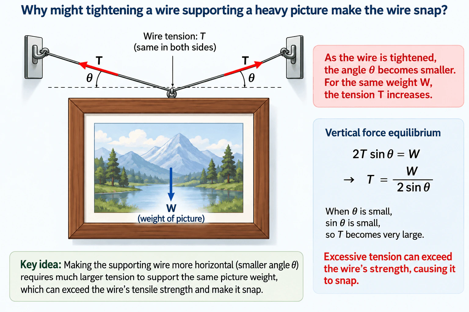
Why might tightening a wire supporting a heavy picture make the wire snap? diagram
How to Explain It in an Interview

Start by defining the free body: the picture has weight W acting downward, and the two wire segments exert tensions T along the wires. State that the setup is symmetric and static. Resolve each wire tension vertically, giving T sin θ. The two vertical components must support the picture, so 2T sin θ = W. Rearranging gives T = W / (2 sin θ). Then explain the physical result: tightening makes the wire more horizontal, which reduces θ and increases the required tension. If that tension becomes greater than the wire's tensile capacity, the wire can snap. Before applying the simplified model to a real installation, verify the actual geometry, wire properties, cross-sectional area, attachment condition, and appropriate design margin.

Technical Approach
  1. Define the free-body boundary around the picture and its supporting connection.
  2. Assume static equilibrium and, for the basic model, two symmetric wire segments carrying equal tension T.
  3. Define W as the picture's weight and θ as each wire segment's angle from the horizontal.
  4. Resolve each tension into horizontal and vertical components.
  5. Use symmetry to show that the horizontal components cancel.
  6. Apply vertical equilibrium: 2T sin θ = W.
  7. Solve for tension: T = W / (2 sin θ).
  8. Evaluate the limiting behavior as θ decreases: sin θ decreases and T increases.
  9. Compare the required tension with the real wire and connection capacity before making any safety conclusion.
Practical Insights

The main tradeoff is geometric. Making the wire more horizontal reduces visible sag, but it sharply increases the tension needed to support the same picture weight. A steeper wire angle reduces the required tension. The simplified model assumes static, symmetric loading and does not include effects such as impact loading, fatigue, damaged wire, weak attachments, or unequal load sharing.

Why Interviewers Ask This

This tests whether the candidate can construct a simple free-body model, resolve inclined forces into components, apply static equilibrium, interpret a limiting case, and connect calculated tension to a realistic tensile failure mode.

Common interview mistakes

Common mistakes are assuming each wire tension is simply W/2, forgetting that only the vertical component T sin θ supports the weight, measuring θ from the wrong reference direction, using cosine when θ is defined from the horizontal, confusing required tension with material strength, and assuming that a simplified equilibrium calculation alone proves a real installation is safe.

Interview tip

Define θ explicitly from the horizontal and write 2T sin θ = W before discussing failure. Then use the limiting case θ → 0° to explain the physics clearly: a nearly horizontal wire needs extremely large tension to provide enough vertical support.
Interviewer may ask next
What assumptions does T = W / (2 sin θ) rely on, and how would you validate them?

It assumes static equilibrium, two symmetric wire segments, equal tension on both sides, and θ measured from the horizontal. I would verify the actual geometry, check that the picture is not undergoing significant dynamic motion, inspect the wire and attachments, and compare the calculated tension with appropriate wire and connection capacities. If the geometry is asymmetric, I would use separate equilibrium equations for the two wire tensions instead of assuming they are equal.

What happens if the wire angle is made steeper instead of more horizontal?

If θ is measured from the horizontal, making the wire steeper increases θ and therefore increases sin θ. From T = W / (2 sin θ), the required tension decreases for the same picture weight. The tradeoff is that a steeper wire generally requires more vertical space or greater visible sag, but mechanically it reduces the tension in each wire segment.

2. Which three factors determine the torque produced by a force about a pivot?Engineering MechanicsEasy

Short Interview Answer (30-60 seconds)

The three factors are the magnitude of the force, the distance from the pivot to the point where the force is applied, and the angle between the position vector and the force. Torque magnitude is τ = rF sin θ. A larger force or a larger effective moment arm produces more torque, while only the component of force perpendicular to the position vector contributes to torque.

Detailed Explanation

Torque describes the turning effect of a force about a pivot. Its magnitude is given by τ = rF sin θ, where r is the distance from the pivot to the point where the force is applied, F is the force magnitude, and θ is the angle between the position vector and the force.

The three determining factors are:

  1. Force magnitude, F: Increasing the force increases the torque when the other factors remain unchanged.
  2. Distance from the pivot, r: Applying the force farther from the pivot increases the torque when the force magnitude and angle remain unchanged.
  3. Force direction, θ: Only the component of the force perpendicular to the position vector creates torque. The sin θ term accounts for this directional effect.

An equivalent expression is τ = Fd⊥, where d⊥ is the perpendicular distance from the pivot to the force's line of action. This perpendicular distance is the moment arm.

The SI unit of torque is newton-metre, N·m. Torque also has a rotational direction. In a planar problem, a consistent sign convention can be chosen, such as counterclockwise positive and clockwise negative.

A useful limiting-case check is the angle. If θ = 90°, then sin θ = 1, so the torque magnitude is maximum for the given r and F. If θ = 0° or 180°, the force's line of action passes through the pivot, so the torque is zero.

Useful Questions to Ask the Interviewer
  • Are you asking for torque magnitude only, or should I also state the clockwise or counterclockwise direction?
  • Is the given distance measured from the pivot to the point of force application, or is it already the perpendicular moment arm?
  • Is this a two-dimensional problem, or should I use the full vector cross product?
How to Explain It in an Interview

I would start with τ = rF sin θ and define the three factors immediately: force magnitude, distance from the pivot, and the angle between the position vector and force. I would explain that the sine term means only the perpendicular component of the force creates the turning effect. I would finish with two quick checks: a perpendicular force gives the maximum torque for a given r and F, while a force whose line of action passes through the pivot gives zero torque.

Technical Approach
  1. Identify the pivot or axis about which torque is required.
  2. Define the position vector r from the pivot to the point where the force is applied.
  3. Determine the force magnitude F and its direction.
  4. Find the angle θ between r and F.
  5. Calculate the torque magnitude using τ = rF sin θ, or equivalently τ = Fd⊥.
  6. Apply the chosen sign convention to identify the rotational direction when required.
  7. Check units and limiting cases, such as θ = 0° and θ = 90°.
Practical Insights

The same torque can be produced by different combinations of force, distance, and direction. For example, when the force is perpendicular to the lever arm, a smaller force can produce the same torque if it acts farther from the pivot. Force direction also matters because a perpendicular force is most effective, while a force whose line of action passes through the pivot produces no torque. In real mechanical systems, increasing the lever arm may be limited by available space, structural stiffness, or geometry.

Why Interviewers Ask This

Interviewers ask this to check whether you understand torque from first principles rather than treating it as a function of force alone. They want to see that you recognize how the force magnitude, the distance from the pivot, and the force direction together determine the turning effect.

Common interview mistakes

Common mistakes are using τ = rF without accounting for the force angle, confusing the direct distance r with the perpendicular moment arm d⊥, using an inconsistent clockwise or counterclockwise sign convention, and forgetting that a force whose line of action passes through the pivot produces zero torque.

Interview tip

State τ = rF sin θ first, define all three factors clearly, and mention the two limiting cases: a perpendicular force gives maximum torque for fixed r and F, while a force whose line of action passes through the pivot gives zero torque. That demonstrates both formula knowledge and physical understanding.

Interviewer may ask next
How would you verify that a calculated torque is reasonable?

Check that the units are force times distance, such as N·m, verify the chosen clockwise or counterclockwise sign convention, and test limiting cases. The torque should become zero when the force's line of action passes through the pivot and should reach rF in magnitude when the force is perpendicular to the position vector.

If you need the same torque but can apply only half as much force, what can you change?

If the force remains perpendicular to the lever arm, you can double the perpendicular moment arm because τ = Fd⊥. More generally, you can increase the distance from the pivot or change the force direction to increase the perpendicular component's effectiveness, subject to the geometry and structural constraints of the system.

3. Why does extending a wrench with a pipe help loosen a tight bolt?Engineering MechanicsEasy

Short Interview Answer (30-60 seconds)

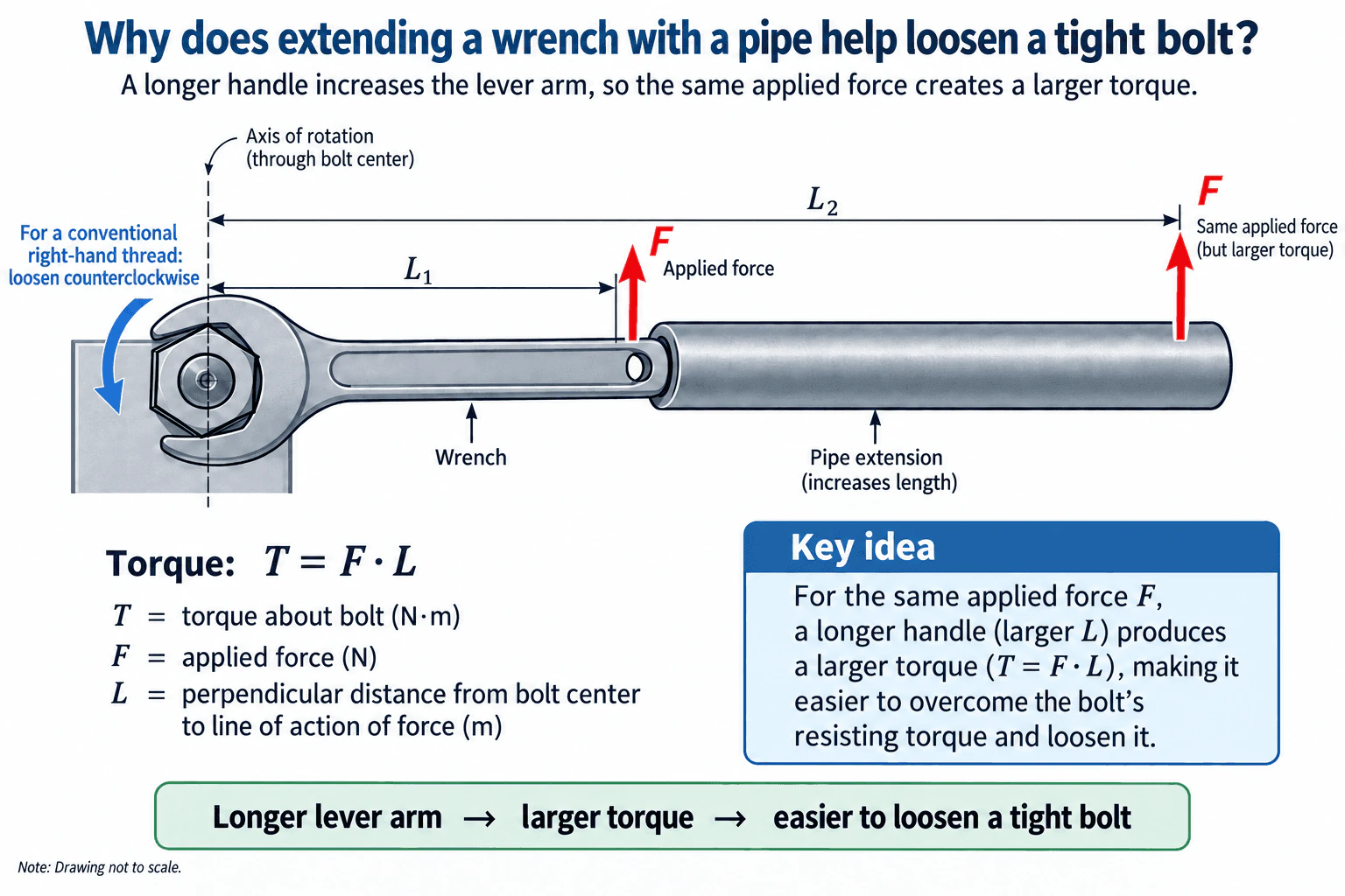
A pipe makes the wrench effectively longer, increasing the lever arm from the bolt center to the applied force. For a perpendicular force, torque is T = F·L. So if the force stays the same but L becomes larger, the torque increases. That greater torque makes it easier to overcome the bolt's resisting or breakaway torque and start loosening it.

Detailed Explanation

A wrench turns a bolt because an applied force creates a moment, or torque, about the bolt's axis of rotation. The important quantity is both the force and the perpendicular distance from the bolt center to the force's line of action.

For a force applied perpendicular to the wrench handle:

T = F·L

where:

  • T = torque about the bolt axis, in N·m
  • F = applied force, in N
  • L = perpendicular distance from the bolt center to the force's line of action, in m

Assume the wrench and pipe act as a rigid body and the force is applied perpendicular to the handle. With the original wrench, the lever arm is L₁, so the applied torque is:

T₁ = F·L₁

With a pipe extension, the same force can be applied farther from the bolt center at lever arm L₂, where L₂ > L₁. The new torque is:

T₂ = F·L₂

Therefore, for the same applied force:

T₂ > T₁

Before the bolt moves, the applied torque is resisted by the fastener and its contact interfaces. Once the applied torque exceeds the required breakaway torque, the bolt can begin rotating. For a conventional right-hand thread, loosening is counterclockwise when viewed from the bolt head. If the wrench extends to the right of the bolt center, an upward perpendicular force produces that counterclockwise moment.

The simple equation T = F·L applies directly when the force is perpendicular to the handle. More generally, torque magnitude is T = rF sin(θ), where θ is the angle between the position vector and the force. This shows why the perpendicular component of force is what produces the turning effect.

A dimensional check also supports the equation: newtons multiplied by metres gives N·m, the unit of torque. A limiting-case check gives the same physical result: applying a force very close to the bolt center produces little torque, while applying the same force farther away produces more torque.

Useful Questions to Ask the Interviewer
  • Should I assume the applied force is perpendicular to the wrench? This determines whether the simple relation T = F·L can be used directly.
  • Should I assume a conventional right-hand-threaded bolt? If so, counterclockwise rotation loosens it when viewed from the bolt head.
  • Should I treat the wrench and pipe as rigid for the conceptual analysis? That is appropriate for the basic statics model, although real tools can deform or fail if overloaded.
Why does extending a wrench with a pipe help loosen a tight bolt? diagram
How to Explain It in an Interview

Start with the physical idea: extending the wrench increases the lever arm. Then write T = F·L for a perpendicular force and define each symbol. Compare T₁ = F·L₁ with T₂ = F·L₂. Because L₂ is greater than L₁, the same force produces greater torque. Conclude that the larger torque makes it easier to exceed the bolt's resisting breakaway torque. Also state the force direction and thread-direction assumption when relevant. Finally, distinguish the mechanics principle from real-world tool safety: a longer extension can also increase loads on the wrench, fastener, and surrounding components.

Technical Approach
  1. Choose the bolt center as the axis of rotation.
  2. Treat the wrench and pipe as one rigid body for the conceptual model.
  3. Identify the applied external force and its direction.
  4. Determine the perpendicular lever arm L from the bolt center to the force's line of action.
  5. For a perpendicular force, calculate torque with T = F·L.
  6. For the original wrench, write T₁ = F·L₁.
  7. For the extended wrench, write T₂ = F·L₂.
  8. Since L₂ > L₁, conclude that T₂ > T₁ for the same force.
  9. Check the moment direction to confirm it acts in the intended loosening direction.
  10. Recognize that actual tool strength, fastener condition, and safe-use limits require separate real-world validation.
Practical Insights

The mechanical advantage comes from increasing the lever arm, not from creating extra force. A longer lever arm lets the same hand force produce more torque, or allows the same required torque to be produced with less hand force. The tradeoff is that greater torque also increases mechanical loading on the wrench, pipe, bolt, and connected parts. The rigid-body torque equation explains the turning effect but does not by itself prove that the tools or fastener can safely withstand the load.

Why Interviewers Ask This

Interviewers are checking whether the candidate understands torque, lever arms, force direction, free-body reasoning, and mechanical advantage. A strong answer should explain why increasing the perpendicular distance from the rotation axis increases torque instead of only saying that a longer wrench gives more leverage.

Common interview mistakes

Common mistakes are saying the pipe creates more force rather than more torque, measuring the lever arm from the wrong point, ignoring the force direction or angle, using T = F·L when the force is not perpendicular without accounting for the angle, confusing force with torque, and assuming that a longer extension is automatically safe for the wrench or fastener.

Interview tip

Use the simple comparison T₁ = F·L₁ and T₂ = F·L₂. Then state that L₂ > L₁, so T₂ > T₁ for the same perpendicular force. This directly connects the longer handle to the larger torque and shows that you understand the mechanics rather than relying on the vague phrase 'more leverage.'

Interviewer may ask next
What changes if the force is not applied perpendicular to the wrench?

The full force no longer contributes to torque. The torque magnitude is T = rF sin(θ), where θ is the angle between the position vector from the bolt center to the force application point and the force direction. Torque is maximum at 90°. As the force becomes more aligned with the wrench, sin(θ) decreases, so the turning effect decreases. Equivalently, the torque can be calculated using the perpendicular distance from the bolt center to the force's line of action.

If you double the effective wrench length while applying the same perpendicular force, what happens to the torque?

The torque doubles. From T = F·L, if the force F stays constant and the lever arm changes from L to 2L, the torque changes from F·L to F·2L = 2F·L. Conversely, if the required torque stays the same, doubling the lever arm ideally reduces the required perpendicular force by half.

4. What kinds of stress arise when a wooden rod is pushed inward or pulled outward at its ends?Engineering MechanicsEasy

Short Interview Answer (30-60 seconds)

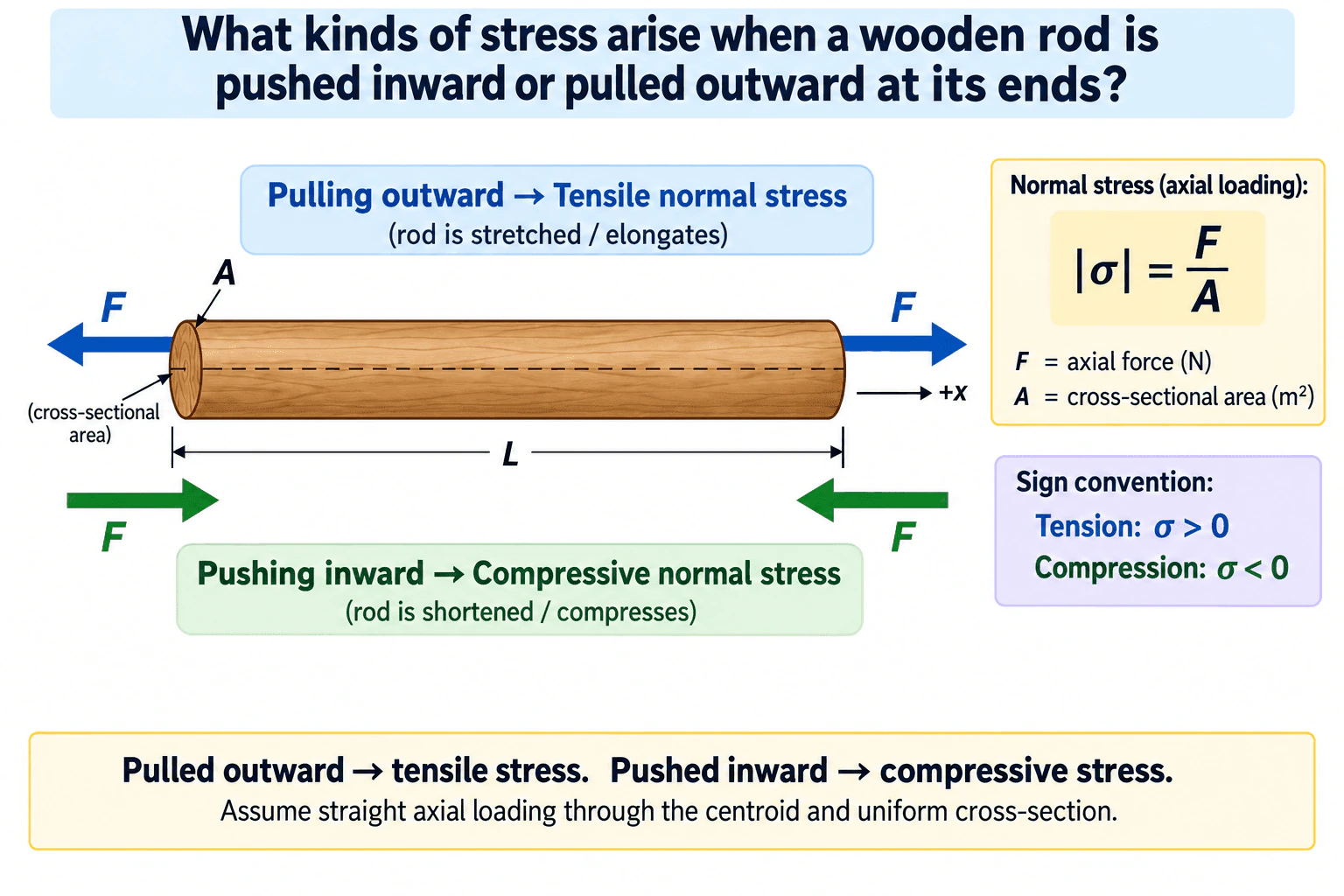
When the wooden rod is pulled outward at both ends, it develops tensile normal stress and tends to elongate. When it is pushed inward at both ends, it develops compressive normal stress and tends to shorten. For a straight rod with a uniform cross-sectional area A and a centered axial force F, the stress magnitude is |σ| = F/A. Using the sign convention shown in the diagram, tension is positive and compression is negative.

Detailed Explanation

A wooden rod loaded along its longitudinal axis develops normal axial stress. Pulling the two ends away from the rod creates tensile normal stress, while pushing the two ends toward the rod creates compressive normal stress.

For the straight, uniform rod shown in the diagram, the average normal-stress magnitude is:

|σ| = F/A

where:

  • σ is the normal stress, measured in pascals (Pa or N/m²),
  • F is the magnitude of the axial force in newtons (N), and
  • A is the cross-sectional area perpendicular to the rod axis in square metres (m²).

Using the sign convention shown in the final diagram:

  • tensile stress: σ > 0,
  • compressive stress: σ < 0.

The rod has a longitudinal +x direction and a length L. Equal and opposite axial forces pointing outward from the rod ends produce tension, so the rod tends to stretch or elongate. Equal and opposite axial forces pointing inward toward the rod ends produce compression, so the rod tends to shorten.

This result assumes a straight rod, a uniform cross-section, and axial loading applied through the centroid. Under those assumptions, the simple F/A relation represents the average normal stress and the load does not intentionally create bending or torsion. Stress should also be kept separate from strain: stress is internal force per unit area, while strain describes relative deformation.

Useful Questions to Ask the Interviewer
  • Should I assume the rod is straight, has a uniform cross-section, and is loaded through its centroid?
  • Are you asking only for the basic axial stress state, or should I also mention buckling for a slender rod in compression?
  • Should I use the sign convention shown here, with tension positive and compression negative?
What kinds of stress arise when a wooden rod is pushed inward or pulled outward at its ends? diagram
How to Explain It in an Interview

I would first identify the wooden rod as an axially loaded member. If the end forces point away from the rod, the rod is in tension and carries tensile normal stress. If the end forces point toward the rod, the rod is in compression and carries compressive normal stress. For a centered axial force on a uniform cross-section, the average stress magnitude is |σ| = F/A. I would then state the sign convention, tension positive and compression negative, and mention that this simple model assumes straight axial loading through the centroid. If the loading were eccentric, bending could also be introduced, and if the compressed rod were very slender, buckling could become important.

Technical Approach

1. Isolate the wooden rod as the free body and identify its longitudinal +x axis. 2. Identify the direction of the equal and opposite axial end forces. 3. If the forces point outward from the rod, classify the loading as axial tension and the resulting normal stress as tensile. 4. If the forces point inward toward the rod, classify the loading as axial compression and the resulting normal stress as compressive. 5. For a straight rod with uniform cross-sectional area A and centered axial loading, calculate the average stress magnitude using |σ| = F/A. 6. Apply the stated sign convention: tension has σ > 0 and compression has σ < 0. 7. Confirm that the load passes through the centroid and that no additional bending, torsion, or instability check is required for the situation being analyzed.

Practical Insights

The basic classification is straightforward for pure axial loading: outward pulling gives tension and inward pushing gives compression. The F/A relation gives average normal stress for a centered axial force on a uniform cross-section. If the geometry is nonuniform, the load is eccentric, or the rod has local notches or holes, the stress may not be uniform. Under compression, a long slender rod can also buckle, so simple compressive stress may not be the only design concern. The amount of deformation depends on material stiffness and is a separate question from identifying the stress state.

Why Interviewers Ask This

Interviewers use this question to check whether you can recognize basic axial loading, distinguish tensile normal stress from compressive normal stress, apply the average normal-stress relationship correctly, and use a consistent stress sign convention without confusing stress with strain or deformation.

Common interview mistakes

Common mistakes include reversing tension and compression, calling the axial stress shear stress, confusing stress with strain, forgetting that A is the cross-sectional area perpendicular to the rod axis, mixing signed stress with stress magnitude, using F/A without stating the axial-loading assumptions, and discussing bending, torsion, fatigue, or buckling as though they are automatically present in a simple centered axial-load case.

Interview tip

Start with the force directions before giving the equation: forces pulling away from the rod mean tension, and forces pushing toward the rod mean compression. Then state |σ| = F/A, define F and A, and give the sign convention. Mention the straight, uniform, centroidal axial-loading assumption to show sound engineering judgment without overcomplicating an easy conceptual question.

Interviewer may ask next
What assumption should you check before using |σ| = F/A for this rod?

Check that the rod is straight, has a reasonably uniform cross-section, and is loaded axially through the centroid. Under those conditions, F/A represents the average normal-stress magnitude. If the force is eccentric or the geometry changes significantly, bending or local stress concentrations may also need to be considered.

What additional concern arises if the wooden rod is long and slender and is pushed inward?

A long, slender rod in compression may become unstable and buckle. In that case, checking only the compressive stress magnitude F/A is not enough; the member length, end boundary conditions, cross-sectional stiffness, and material stiffness also affect its buckling resistance.

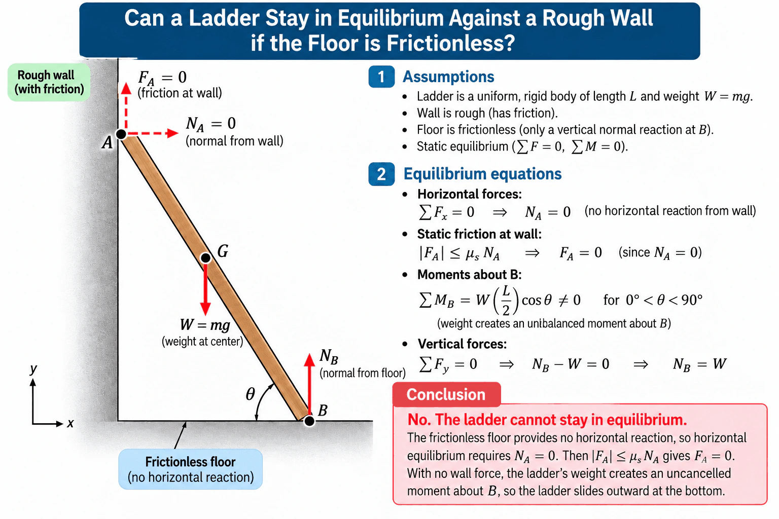
5. Can a ladder stay in equilibrium against a rough wall if the floor is frictionless?Engineering MechanicsMedium

Short Interview Answer (30-60 seconds)

No. A frictionless floor supplies only a vertical reaction at the bottom. With no horizontal floor reaction, horizontal equilibrium requires the wall normal force N_A to be zero. Because |F_A| ≤ μ_s N_A, the available wall friction F_A is also zero. The floor reaction can balance the weight vertically, but the weight still creates a nonzero moment about the bottom contact B. Therefore the leaning ladder cannot remain in static equilibrium and its bottom slides outward.

Detailed Explanation

The key is to start with the support conditions and then apply all three planar rigid-body equilibrium equations.

Assume a uniform rigid ladder of length L and weight W = mg. Its bottom contact B is on a frictionless horizontal floor, and its top contact A touches a rough vertical wall. Let θ be the angle between the ladder and the floor, with 0° < θ < 90°. The ladder's weight W acts downward at its midpoint G.

At B, the frictionless floor can provide only the upward normal reaction N_B. It cannot provide a horizontal friction force. At A, the wall could in principle provide a horizontal normal reaction N_A and a vertical static-friction force F_A.

Apply horizontal equilibrium:

ΣF_x = 0 ⇒ N_A = 0.

Because static friction at the wall is limited by

|F_A| ≤ μ_s N_A,

and N_A = 0, it follows that

F_A = 0.

Now apply vertical equilibrium:

ΣF_y = 0 ⇒ N_B - W = 0 ⇒ N_B = W.

So the vertical forces can balance. However, force balance alone is not sufficient for rigid-body equilibrium. The moment equation must also be satisfied.

Take moments about B. The reaction N_B passes through B, so it produces no moment about B. Since N_A = 0 and F_A = 0, there is no wall force to oppose the moment caused by the ladder's weight. For a uniform ladder, the weight acts at L/2 from B, giving the moment magnitude

W(L/2)cosθ.

For 0° < θ < 90°, cosθ is nonzero, so

ΣM_B = W(L/2)cosθ ≠ 0.

Therefore the ladder cannot satisfy static equilibrium. The bottom moves outward while the top moves downward. This matches the approved diagram's force relationships: N_A = 0, F_A = 0, N_B = W, and a nonzero moment about B.

Useful Questions to Ask the Interviewer
  • Should I assume the ladder is uniform and rigid? For a uniform ladder, its weight acts at the midpoint.
  • Is the floor perfectly frictionless? If yes, the bottom contact has no horizontal reaction.
  • Should I use the ordinary Coulomb static-friction model at the wall? If yes, wall friction is limited by |F_A| ≤ μ_s N_A.
  • Should I assume the ladder is genuinely leaning, so 0° < θ < 90°? The exactly vertical position θ = 90° is a limiting special case.
Can a ladder stay in equilibrium against a rough wall if the floor is frictionless? diagram
How to Explain It in an Interview

Start with the boundary condition at the floor. Because the floor is frictionless, it cannot supply a horizontal reaction. Therefore horizontal equilibrium forces N_A = 0 at the wall. Once N_A is zero, the wall cannot develop static friction either, because |F_A| ≤ μ_s N_A, so F_A = 0. Vertical equilibrium gives N_B = W, but the weight still creates an uncancelled moment about B equal in magnitude to W(L/2)cosθ. For a leaning ladder that moment is nonzero, so static equilibrium is impossible. The important insight is that making the floor frictionless removes the horizontal force needed to develop a wall normal reaction, and without that normal reaction the rough wall cannot provide friction.

Technical Approach

1. Isolate the ladder as one rigid-body free body. 2. Define the contacts: A at the rough wall and B at the frictionless floor. 3. Identify the possible reactions: N_A horizontally at A, F_A vertically at A, and N_B vertically at B. 4. Use horizontal equilibrium: ΣF_x = 0 ⇒ N_A = 0. 5. Apply the static-friction constraint: |F_A| ≤ μ_s N_A ⇒ F_A = 0. 6. Use vertical equilibrium: ΣF_y = 0 ⇒ N_B = W. 7. Take moments about B. The floor reaction has zero moment about B, and both wall reactions are zero. 8. The remaining weight produces moment magnitude W(L/2)cosθ. 9. For 0° < θ < 90°, that moment is nonzero, so ΣM_B = 0 cannot be satisfied. 10. Conclude that the leaning ladder cannot remain in static equilibrium.

Practical Insights

The result depends on the support boundary conditions rather than simply on how rough the wall is. A larger coefficient of static friction does not help when the wall normal reaction is zero, because the maximum available wall friction is proportional to N_A. If the floor could provide friction, it could supply a horizontal reaction, allowing a nonzero N_A and potentially allowing equilibrium. The conclusion here assumes an ordinary rigid ladder, Coulomb static friction, and a leaning angle with 0° < θ < 90°.

Why Interviewers Ask This

This tests whether the candidate can build a correct free-body diagram, apply both force and moment equilibrium, understand that static friction depends on the normal reaction, and recognize how a support boundary condition can make equilibrium impossible.

Common interview mistakes

Common mistakes include adding a horizontal reaction at the frictionless floor, assuming that a rough wall automatically provides a nonzero friction force, calculating F_A as nonzero after finding N_A = 0, checking only ΣF_x = 0 and ΣF_y = 0 without checking moments, or saying the failure is caused by an inability to balance the vertical forces. In fact, N_B = W can balance the weight vertically; equilibrium fails because the weight still produces an uncancelled moment about B.

Interview tip

State the support constraints first. A strong compact explanation is: 'The frictionless floor cannot provide a horizontal reaction, so horizontal equilibrium requires the wall normal N_A to be zero. That also forces the wall friction F_A to zero. The floor reaction can balance W vertically, but the weight still produces a nonzero moment about B. Therefore the leaning ladder cannot be in static equilibrium.'

Interviewer may ask next
Would making the wall extremely rough allow the ladder to stay in equilibrium?

No. The available static friction satisfies |F_A| ≤ μ_s N_A. Since horizontal equilibrium requires N_A = 0 when the floor is frictionless, μ_s N_A is zero for any finite coefficient of friction. Therefore the wall still cannot provide a nonzero friction force.

What changes if the floor is also rough?

A rough floor can provide a horizontal friction force at B. That force can balance a nonzero wall normal reaction N_A, which in turn allows the wall to develop a friction force. Static equilibrium can then be possible, provided the required friction forces at the contacts remain within their respective static-friction limits.

6. Which methods do you use to estimate a structure’s fatigue life?Engineering MechanicsHard

Short Interview Answer (30-60 seconds)

I first determine the cyclic stress or strain history at the fatigue-critical location and decide which physical fatigue regime applies. For predominantly elastic, high-cycle behavior, I use the stress-life or S-N method. When local cyclic plasticity is significant, I use the strain-life or ε-N method. If an initial crack or flaw must be considered, I use fracture-mechanics crack-growth analysis. For variable-amplitude loading, I identify cycles, account for mean stress, and may use a cumulative-damage model such as Miner’s rule. I also account for geometry, stress concentrations, surface and environmental effects when supported by appropriate data, and validate the prediction against relevant material, component, inspection, or test evidence.

Detailed Explanation

Fatigue-life estimation starts with the loading at the location where fatigue damage is most likely to occur. I do not choose a fatigue equation until I understand the load path, boundary conditions, cyclic stress or strain range, mean load, number and sequence of cycles, geometry, operating environment, and whether an initial crack must be considered.

The main methods I use are:

  1. Stress-life, or S-N, method. I use this primarily when the local deformation is predominantly elastic and the expected life is relatively high. An S-N curve relates cyclic stress amplitude or stress range to cycles to failure for a defined material and test condition. I determine the cyclic stress at the critical location, include an appropriate mean-stress treatment when needed, and compare it with fatigue data that represent the material and service condition as closely as practical.
  1. Strain-life, or ε-N, method. I use this when local cyclic plasticity is significant, such as near a notch under larger cyclic loads or during low-cycle fatigue. The total strain amplitude is represented by elastic and plastic contributions. A common strain-life relationship combines the Basquin elastic term and Coffin-Manson plastic term. This approach is more appropriate than a purely elastic S-N calculation when the local response includes repeated plastic strain.
  1. Fracture-mechanics crack-growth method. If a known or assumed initial flaw must be considered, I estimate the stress-intensity-factor range, ΔK, and use suitable crack-growth data. In a region where a Paris-type relationship is applicable, crack growth may be represented by da/dN = C(ΔK)^m, where a is crack size, N is cycles, and C and m are material constants for the specified conditions. Integrating the crack-growth relation from an initial crack size ai to an appropriate critical crack size ac gives an estimate of propagation life. This method predicts crack-growth life rather than assuming that the structure begins without a flaw.
  1. Variable-amplitude fatigue analysis. Real structures often see irregular loading rather than one constant stress amplitude. I obtain or estimate the load-time history, convert the loads into local stresses or strains, and identify cycles using an appropriate cycle-counting method such as rainflow counting. I then combine the damage from different cycle ranges using a suitable cumulative-damage model when justified.

A common simplified cumulative-damage method is Miner’s rule. If ni cycles occur at a particular stress level and the corresponding constant-amplitude fatigue data predict Ni cycles to failure at that level, the damage fraction is ni/Ni. The accumulated damage is D = Σ(ni/Ni). A nominal failure condition is often associated with D near 1 in the idealized linear model, but actual fatigue damage can differ because Miner’s rule does not fully represent load-sequence effects, overload interactions, residual-stress changes, or other nonlinear behavior.

Mean stress also matters. Two cycles with the same alternating stress can produce different fatigue behavior if their mean stresses differ. Depending on the material data and the adopted fatigue method, I may use a mean-stress correction such as Goodman, Gerber, or another relationship appropriate to the application. I would not automatically apply a particular correction without checking that it is compatible with the material data and design method.

Geometry is another major input. I first establish nominal stresses from the actual axial forces, bending moments, torsion, and other relevant loads using the correct boundary conditions. At features such as holes, shoulders, threads, fillets, or other discontinuities, nominal stress alone may be insufficient. I evaluate the local stress concentration and distinguish the theoretical elastic stress-concentration factor Kt from fatigue-specific notch behavior, such as a fatigue notch factor Kf when that concept is appropriate. For welded structures, the applicable fatigue procedure may instead use nominal stress, structural or hot-spot stress, or another weld-specific method defined by the governing design approach.

For complex geometry, finite-element analysis can help determine local elastic or elastic-plastic stress and strain. However, FEA only provides the mechanical response; a fatigue-life prediction still requires a suitable fatigue model, material data, load history, and interpretation of local stresses or strains.

I also check whether the available fatigue data represent the actual service conditions closely enough. Surface condition, component size, manufacturing condition, residual stress, weld condition, corrosion, temperature, and environment can influence fatigue performance. I include these effects only through defensible data, testing, or an applicable engineering method rather than inventing correction factors.

When fracture mechanics is used, I also check whether the selected crack-growth relation is valid over the relevant ΔK range. Near the crack-growth threshold or near final fracture, a simple Paris-law region may not adequately represent the behavior. The critical crack size must also be based on appropriate fracture mechanics, material toughness, geometry, and loading rather than chosen arbitrarily.

I validate the result by checking units, signs, equilibrium, principal or equivalent stresses where relevant, the fatigue-critical location, and mesh sensitivity if FEA is used. Because fatigue life can change greatly with relatively small changes in local stress or strain, I perform sensitivity checks on uncertain loads, stress concentrations, material data, and other influential inputs. For an actual design decision, I compare the analytical prediction with appropriate fatigue data, component testing, inspection information, applicable standards, or validated field evidence rather than declaring the structure safe from a simplified calculation alone.

Useful Questions to Ask the Interviewer
  • Is the loading constant-amplitude or variable-amplitude, and do we have a measured or specified load history?
  • Is the expected local response predominantly elastic, or is cyclic plasticity expected?
  • Are we estimating total life from an initially uncracked condition, or propagation from a known or assumed flaw?
  • Do we have material S-N, strain-life, or crack-growth data for the relevant material condition, temperature, surface condition, and environment?
  • Are there welds, holes, fillets, threads, or other stress concentrations at the likely fatigue-critical location?
  • Is there a governing design standard, inspection requirement, target reliability, or required design life?
How to Explain It in an Interview

I would explain that I do not use one fatigue model for every structure. I begin with the actual cyclic load history and determine the stress or strain response at the fatigue-critical location. If the local response is predominantly elastic and high-cycle, I use an S-N approach. If cyclic plasticity is significant, I use an ε-N approach. If an initial crack must be considered, I use fracture-mechanics crack-growth analysis. For variable-amplitude loading, I identify cycles, account for relevant mean-stress effects, and use an appropriate cumulative-damage model where justified. I then account for geometry, service conditions, and uncertainty using defensible data and validate the prediction against material data, testing, inspection evidence, and applicable engineering requirements. The key is to choose the method that matches the actual fatigue mechanism and the quality of the available inputs.

Technical Approach
  1. Define the structure, free-body boundary, supports, load path, coordinates, units, operating environment, and required service history.
  2. Separate static loads from cyclic and dynamic loads and determine the time-dependent forces and moments that drive fatigue.
  3. Calculate nominal stresses or strains and identify likely fatigue-critical locations.
  4. Evaluate local stress or strain concentrations using analytical methods, validated FEA, or appropriate test data.
  5. Classify the problem as primarily stress-life, strain-life, or crack-growth fatigue based on whether the local response is predominantly elastic, includes significant cyclic plasticity, or requires an initial flaw to be considered.
  6. Obtain fatigue data appropriate to the material, geometry or detail category, temperature, surface or weld condition, and environment.
  7. For variable-amplitude loading, convert the load history into stress or strain cycles using an appropriate cycle-counting method such as rainflow counting.
  8. Account for mean stress and other justified modifiers or detail effects using a method compatible with the selected fatigue data.
  9. Estimate life using the applicable S-N, ε-N, cumulative-damage, or fracture-mechanics model. For crack growth, calculate ΔK as a function of crack size and integrate an appropriate da/dN relation from the initial crack size to an applicable limiting crack size.
  10. Check units, equilibrium, boundary conditions, sign conventions, model applicability, and sensitivity to uncertain loads, geometry, and material properties.
  11. Compare predicted critical locations and life with suitable test, inspection, or field evidence where available.
  12. Use the prediction together with applicable design standards, inspection planning, required reliability, and engineering judgment rather than treating the calculated life alone as proof of structural safety.
Practical Insights

The main tradeoff is between model simplicity and physical detail. An S-N calculation is efficient when the local response is mostly elastic and suitable fatigue data are available, but it does not directly represent significant cyclic plasticity. A strain-life analysis represents local elastic-plastic behavior better but requires additional material properties and a reliable estimate of local strain. Crack-growth analysis is appropriate when flaws and damage tolerance matter, but it requires crack-size information, stress-intensity calculations, fracture properties, and crack-growth data. Variable-amplitude loading adds uncertainty because cycle sequence and overloads can influence real damage differently from a simple linear accumulation model. FEA can improve the estimate of local stress or strain in complex geometry, but a detailed model cannot compensate for incorrect loads, boundary conditions, mesh interpretation, or fatigue material data. Fatigue predictions also contain material scatter and can be sensitive to manufacturing condition, residual stress, surface condition, environment, and local geometry, so validation and appropriate design margins remain important.

Why Interviewers Ask This

Interviewers want to see whether I can select a fatigue-life method that matches the loading regime, material behavior, geometry, stress concentrations, mean stress, and available evidence. They are also testing whether I understand the difference between estimating crack-initiation life and crack-propagation life, and whether I recognize the uncertainty in fatigue calculations rather than treating one simplified equation as a guarantee of service life.

Common interview mistakes

Common mistakes include using only the maximum static stress instead of the cyclic stress or strain range; applying an S-N method where significant local plasticity makes a strain-life method more appropriate; ignoring mean stress when it is relevant; using nominal stress while missing a severe local stress concentration; confusing Kt with fatigue-specific notch behavior; using fatigue data that do not represent the actual material, weld detail, temperature, surface condition, or environment; silently mixing units; treating Miner’s rule as an exact representation of all load-sequence effects; applying the Paris crack-growth law outside the range where it is valid; choosing an arbitrary critical crack size; treating an FEA stress contour as a complete fatigue prediction without a fatigue model; ignoring a known flaw when crack propagation controls life; and claiming a structure is safe solely because a simplified fatigue calculation predicts the desired number of cycles.

Interview tip

Organize the answer around the physical fatigue mechanism. Start with the cyclic load history and fatigue-critical location, then state S-N for predominantly elastic high-cycle behavior, ε-N when cyclic plasticity matters, and fracture mechanics when an existing or assumed flaw must be considered. Add variable-amplitude cycle counting, mean-stress treatment, local stress concentration, relevant service-condition effects, and validation. This shows that you select the method from the mechanics of the problem instead of applying one memorized fatigue equation.

Interviewer may ask next
How would you validate a fatigue-life prediction before relying on it for a real structure?

I would first verify the loads, load history, boundary conditions, units, equilibrium, and the calculated fatigue-critical stress or strain locations. If FEA is involved, I would check reactions, mesh sensitivity, local stress interpretation, and agreement with hand calculations for simpler load paths. I would confirm that the fatigue material data, weld detail data, and any correction methods represent the relevant material and operating condition. I would perform sensitivity studies because fatigue life can change strongly with relatively small changes in local stress or strain. Where appropriate, I would compare the predicted failure location and life with coupon tests, component tests, inspection data, or other validated evidence. Finally, I would apply the relevant design, inspection, and reliability requirements rather than treating the analytical result by itself as certification that the structure is safe.

How would your approach change if inspection found an existing fatigue crack?

I would shift the emphasis from an initiation-based S-N or ε-N estimate to a damage-tolerance and fracture-mechanics approach. I would characterize the crack location, geometry, and measured size, determine the cyclic stress field, calculate the stress-intensity-factor range ΔK as the crack grows, and use suitable crack-growth data to estimate propagation from the detected crack size toward an applicable limiting crack size. I would check whether the selected crack-growth model is valid across the relevant ΔK range and account for variable-amplitude effects with an appropriate model where necessary. I would also evaluate fracture resistance and determine inspection or disposition requirements under the applicable engineering criteria. The remaining-life estimate would depend strongly on crack-size measurement, load history, geometry, fracture properties, and crack-growth data, so those inputs would need careful validation.

7. What must be considered when analyzing thermal stresses?Engineering MechanicsHard

Short Interview Answer (30-60 seconds)

When analyzing thermal stresses, I first determine the temperature distribution and how freely the component can expand or contract. A uniform temperature change in a homogeneous, completely free component produces thermal strain but ideally no thermal stress. Stress develops when expansion is restrained, when temperature varies within the component, or when joined materials have different coefficients of thermal expansion. I also consider the stress-free reference temperature, geometry, supports and interfaces, temperature-dependent material properties, external loads, and whether yielding, creep, or repeated thermal cycling is important. Finally, I check the combined stress state against appropriate strength, fatigue, deformation, and stability limits.

Detailed Explanation

Thermal-stress analysis begins with a simple distinction: a temperature change produces thermal strain, while restraint or incompatibility of that strain produces thermal stress.

For a homogeneous material under a uniform temperature change, the free thermal strain is

ε_th = αΔT

where ε_th is thermal strain, α is the coefficient of thermal expansion, and ΔT is the temperature change from the relevant stress-free reference temperature.

If the component is completely free to expand or contract and the temperature change is uniform, this strain ideally produces no mechanical stress. If a simple one-dimensional elastic member is fully restrained, its total axial strain is zero. The mechanical strain must therefore oppose the free thermal strain:

ε_mech = -ε_th = -αΔT

For linear-elastic behavior,

σ = Eε_mech = -EαΔT

where E is Young's modulus. For heating, this sign convention gives compression under full restraint; for cooling, it gives tension.

The equation σ = -EαΔT is only a special case. A real analysis must establish the actual temperature field, mechanical boundary conditions, geometry, material behavior, and load history before choosing the stress model.

Useful Questions to Ask the Interviewer
  1. Is the temperature change uniform, or is there a temperature gradient through the component?
  2. What temperature represents the stress-free or assembly reference condition?
  3. Is the component free to expand, partially restrained, or fully restrained in each direction?
  4. Are multiple materials joined together, and do they have different coefficients of thermal expansion?
  5. What operating temperature range and thermal-cycle history are expected?
  6. Should the material be treated as linear elastic, or are yielding, creep, relaxation, or other temperature-dependent effects important?
  7. Are external mechanical loads acting at the same time as the thermal loading?
  8. Are local stresses near joints, holes, welds, contacts, or geometric discontinuities important?
How to Explain It in an Interview

I would analyze thermal stress in a structured sequence.

First, I define the thermal loading. I identify the stress-free reference temperature, the operating temperatures, and whether the temperature field is uniform, spatially varying, or transient. A temperature gradient can make different regions of the same component want to expand by different amounts, producing internal stress, bending, or warping even without a simple external axial restraint.

Second, I define the mechanical boundary conditions. I determine which directions are free to expand and which are restrained by supports, joints, contact, adjacent components, or assembly constraints. This is critical because a uniform temperature change in a freely expanding homogeneous part does not by itself create thermal stress.

Third, I use material properties appropriate to the actual temperature. Important properties can include the coefficient of thermal expansion α, Young's modulus E, Poisson's ratio, yield strength, and, when relevant, creep or viscoelastic properties. Over a large temperature range, assuming constant properties may be inaccurate.

Fourth, I determine the free thermal strain. For an appropriate constant-property case, ε_th = αΔT. If α changes significantly with temperature, the thermal strain is more accurately represented by integrating α over the temperature range rather than using one constant value.

Fifth, I apply compatibility and equilibrium. The actual deformation must satisfy the supports, interfaces, and continuity between connected regions. The difference between the strain the material would undergo freely and the strain permitted by the constraints creates mechanical strain, which is converted to stress through the appropriate constitutive relationship.

For example, a uniform, fully restrained, one-dimensional elastic member has zero total axial strain. Its free thermal strain αΔT is opposed by a mechanical strain of -αΔT, giving σ = -EαΔT. If the restraint has finite stiffness instead of being perfectly rigid, both the member and the restraint deform, so the thermal stress is generally smaller and must be found from equilibrium and compatibility.

Sixth, I check for differential expansion between materials. Two bonded materials with different coefficients of thermal expansion would expand by different amounts if they were separate. Because the interface forces them to deform compatibly, internal stresses develop. The resulting stress depends on the stiffness, geometry, thermal-expansion coefficients, temperature change, and constraint conditions of both materials.

Seventh, I consider temperature gradients and geometry. Through-thickness or local temperature gradients can cause thermal bending and multiaxial stresses. Holes, fillets, welds, contacts, sharp geometry changes, and other discontinuities can also increase local stress, so a simple axial equation may no longer be adequate.

Eighth, I verify whether linear elasticity remains valid. At elevated temperature, elastic modulus and strength may decrease. If stresses exceed the elastic range, plastic deformation changes the stress distribution. At sufficiently high temperature and long exposure time, creep can relax or redistribute stresses and can also create permanent deformation.

Ninth, I consider repeated temperature changes. Thermal cycling creates a changing stress range and may cause thermal fatigue even when a single cycle does not produce immediate failure. Local plastic strain, temperature gradients, stress concentrations, and cycle count become important in that assessment.

Tenth, I combine thermal effects with simultaneous mechanical loads. Thermal stress should not automatically be evaluated in isolation if pressure, weight, torque, vibration, or other loads are present. For a multiaxial state, principal stresses or an appropriate failure criterion may be needed.

Finally, I validate the model. I check units, signs, reactions, deformation compatibility, equilibrium, material-property ranges, and limiting cases. A useful limiting check is that restraint-induced stress should approach zero as restraint stiffness approaches zero for a uniformly heated homogeneous component. For critical equipment, simplified calculations should be supported by suitable testing, validated numerical analysis, or applicable engineering standards rather than being treated alone as proof that a design is safe.

Technical Approach
  1. Define the component boundaries, geometry, coordinates, units, and stress-free reference temperature.
  2. Determine the temperature field and whether heating or cooling is uniform, transient, or spatially varying.
  3. Identify supports, contacts, interfaces, and the permitted thermal expansion in each relevant direction.
  4. Obtain material properties at the relevant temperatures, including coefficient of thermal expansion, Young's modulus, Poisson's ratio, and strength properties where applicable.
  5. Calculate the free thermal strain, using ε_th = αΔT for an appropriate constant-property case or a temperature-dependent relation when required.
  6. Apply deformation compatibility and equilibrium to determine how much free thermal deformation is restrained.
  7. Convert the resulting mechanical strain into stress using a constitutive model appropriate to the material and temperature.
  8. Include temperature gradients, dissimilar-material expansion, contact effects, geometric stress concentrations, and simultaneous mechanical loads where relevant.
  9. Check whether yielding, creep, buckling, fatigue, or thermal fatigue changes the governing behavior.
  10. Validate reactions, units, deformation, equilibrium, limiting cases, and assumptions before comparing the combined stress state with appropriate design criteria.
Practical Insights

The simplest case is a uniform temperature change in a straight, linear-elastic member with clearly defined restraint, where thermal strain and stress can be calculated directly. The analysis becomes more difficult when temperature varies across the part, supports have finite stiffness, several materials are joined, properties change with temperature, contact conditions change, or the material yields or creeps. A more detailed analytical or numerical model can capture these effects, but it requires better temperature data, boundary conditions, material properties, and validation. The main tradeoff is between a simple model that is easy to check and a more detailed model that represents the actual component more accurately.

Why Interviewers Ask This

Interviewers want to see whether I understand that temperature change alone does not necessarily create stress. Thermal stress develops when thermal expansion or contraction is restrained, when temperature varies spatially and creates incompatible thermal strains, or when connected materials have different thermal-expansion behavior. They are evaluating whether I can identify the correct boundary conditions, use material properties at the actual operating temperature, distinguish thermal strain from mechanical strain, and recognize when a simple one-dimensional equation is insufficient.

Common interview mistakes

Common mistakes include assuming that every temperature change automatically creates stress, using σ = EαΔT without confirming the full-restraint assumptions, ignoring the stress-free reference temperature, treating a nonuniform temperature field as uniform, using room-temperature material properties at elevated temperature, ignoring differential expansion between joined materials, confusing absolute temperature with temperature change, overlooking creep or yielding at high temperature, ignoring thermal fatigue during repeated cycles, and evaluating thermal stress separately from simultaneous mechanical loads when the combined stress state controls the design.

Interview tip

Start by stating that thermal expansion is not automatically the same as thermal stress. Then organize the answer around temperature distribution, restraint, material properties, compatibility, and failure mechanisms. Use σ = -EαΔT only as the special case of a uniformly heated, fully restrained, one-dimensional linear-elastic member. Explaining both the equation and its assumptions demonstrates stronger engineering judgment than quoting the equation alone.

Interviewer may ask next
How would the result change if the component were free to expand instead of fully restrained?

For an ideal homogeneous component undergoing a uniform temperature change, removing the restraint allows it to develop its free thermal strain ε_th = αΔT, so the restraint-induced thermal stress approaches zero. I would still check for local constraints, contact, temperature gradients, connected components, gravity, and mechanical loads that could prevent completely free deformation. A useful validation is that the calculated restraint-induced stress should tend toward zero as the effective restraint stiffness tends toward zero.

What changes if the component experiences repeated heating and cooling at high temperature?

The problem becomes cyclic and temperature-dependent rather than only a single elastic stress calculation. I would evaluate the temperature range, stress and strain ranges, temperature-dependent material properties, cycle history, and whether local yielding occurs. Repeated expansion and contraction can cause thermal fatigue, especially near stress concentrations or constrained joints. At sufficiently high temperature and long exposure time, creep can also relax or redistribute stress while accumulating permanent deformation. The assessment therefore requires the temperature-time history and suitable fatigue, creep, and combined-load criteria rather than relying only on the peak elastic value from σ = -EαΔT.

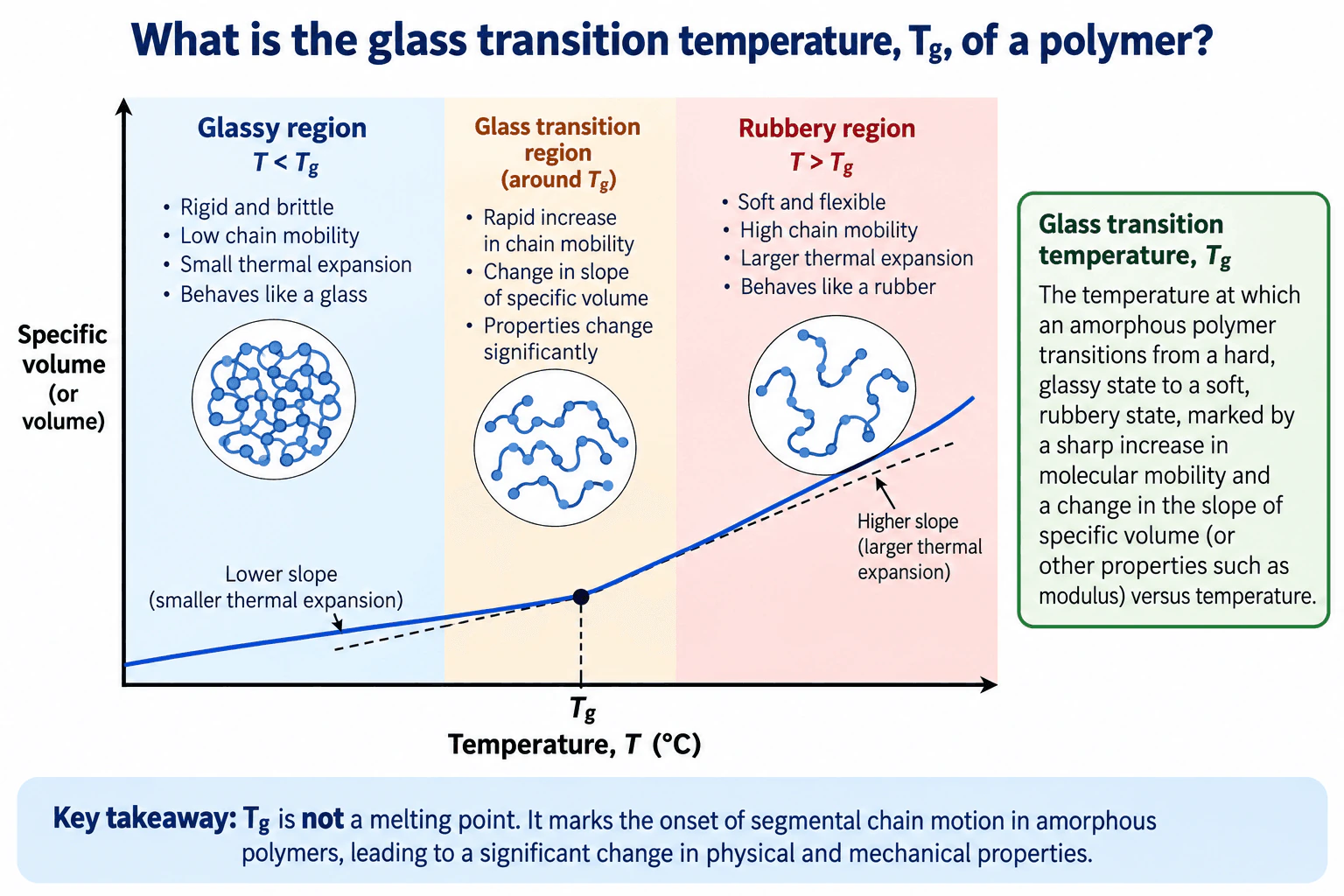
8. What is the glass transition temperature, Tg, of a polymer?Materials And Material SelectionEasy

Short Interview Answer (30-60 seconds)

The glass transition temperature, Tg, is the temperature region where the amorphous portions of a polymer change from a hard, glassy state to a softer, rubbery state as segmental chain mobility increases. Below Tg, chain mobility is low and the polymer is generally rigid and brittle. Above Tg, segmental mobility is higher, so the polymer becomes softer and more flexible and usually shows greater thermal expansion. Tg is not the melting point.

Detailed Explanation

The glass transition temperature, Tg, describes a major change in the behavior of the amorphous regions of a polymer. Below Tg, polymer-chain segments have limited mobility. The material therefore behaves in a glass-like manner and is generally hard, rigid, and relatively brittle.

As the temperature rises through the glass-transition region, segmental molecular motion increases significantly and physical and mechanical properties change. Above Tg, the amorphous polymer has greater segmental chain mobility, so it generally becomes softer and more flexible and behaves more like a rubber.

A common way to identify the transition is with a specific-volume-versus-temperature curve. Specific volume increases as temperature increases. Below Tg, the curve has a lower slope, representing smaller thermal expansion. Around Tg, the slope changes. Above Tg, the slope is higher, representing larger thermal expansion. Other properties, including modulus, also change substantially through the transition.

Tg is not the melting temperature. Glass transition is associated with increased segmental mobility in amorphous polymer material. Melting is a different transition associated with loss of crystalline order. A fully amorphous polymer can therefore exhibit Tg without melting at Tg, while a semicrystalline polymer can have a Tg associated with its amorphous regions and a separate melting temperature for its crystalline regions.

Useful Questions to Ask the Interviewer
  • Are we discussing a fully amorphous polymer or the amorphous regions of a semicrystalline polymer?
  • Is the expected service temperature below, near, or above Tg?
  • Is the important design requirement stiffness, flexibility, dimensional stability, or resistance to brittle behavior?
  • Which measured property or test method is being used to characterize the transition, such as modulus or thermal expansion behavior?
What is the glass transition temperature, Tg, of a polymer? diagram
How to Explain It in an Interview

Start with the physical meaning: Tg is the temperature region where increased segmental chain mobility causes amorphous polymer behavior to change from glassy to rubbery. Then compare the two sides of the transition. Below Tg, mobility is low, so the polymer tends to be rigid and brittle. Above Tg, mobility is higher, so it tends to be softer and more flexible. Next, connect this to a measurable property: on a specific-volume-versus-temperature graph, the slope becomes larger above Tg because thermal expansion is greater. Finish by stating clearly that Tg is not the melting point. For material selection, the key question is whether the service-temperature range lies below, near, or above Tg because that strongly affects stiffness, flexibility, thermal expansion, and dimensional stability.

Technical Approach
  1. Identify the expected service-temperature range.
  2. Determine the relevant Tg for the polymer in its actual material condition.
  3. Compare the service-temperature range with Tg.
  4. For operation below Tg, expect predominantly glassy behavior with low segmental mobility and relatively high rigidity.
  5. Near Tg, expect properties to change significantly with temperature, so this region requires careful evaluation.
  6. Above Tg, expect greater segmental mobility, lower stiffness, greater flexibility, and generally greater thermal expansion.
  7. Validate the material choice using measured property data or testing representative of the intended service conditions.
Practical Insights

The main engineering tradeoff is that the same polymer can behave very differently depending on its temperature relative to Tg. Below Tg, higher rigidity and dimensional stability may be useful, but brittle behavior can become more important. Above Tg, greater flexibility may be useful, but stiffness is reduced and thermal expansion is generally larger. Near Tg, relatively small temperature changes can produce substantial property changes, so the design should use data that represents the actual operating range.

Why Interviewers Ask This

Interviewers want to confirm that you understand how temperature affects polymer behavior and that you can distinguish the glass transition from melting. A strong answer connects Tg to increased segmental chain mobility, the change from glassy to rubbery behavior, and measurable property changes such as the change in slope of specific volume versus temperature.

Common interview mistakes

Common mistakes include calling Tg the melting point, treating Tg as an exact melting-like temperature instead of a transition region, assuming the entire polymer becomes freely mobile above Tg, or ignoring the service temperature relative to Tg. Another mistake is giving only a molecular definition without explaining the engineering consequence: stiffness, flexibility, thermal expansion, and other physical properties can change substantially through the glass-transition region.

Interview tip

Give the definition first, then compare behavior below and above Tg. A strong concise explanation is: below Tg, the amorphous polymer is glassy with low segmental mobility; above Tg, segmental mobility increases and the polymer becomes softer and more rubbery. Add that the specific-volume-versus-temperature curve changes slope around Tg, with a higher slope above Tg, and explicitly state that Tg is not the melting point.

Interviewer may ask next
How would you verify that a polymer is suitable if its operating temperature is close to Tg?

I would not rely on the Tg value alone. I would review measured mechanical and thermal properties over the full service-temperature range and under representative loading and environmental conditions. Near Tg, stiffness, dimensional stability, flexibility, and thermal expansion can change significantly with temperature, so the material should be validated using data or tests that represent the actual application.

What changes if the component must operate above Tg instead of below Tg?

Above Tg, the amorphous regions have greater segmental chain mobility, so the polymer generally becomes softer and more flexible. Its modulus is typically lower and its thermal expansion is generally greater than below Tg. If the design requires high rigidity or tight dimensional stability, operation above Tg may therefore be unsuitable unless the selected polymer system still meets those requirements at the actual service temperature.

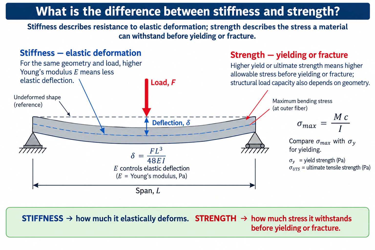
9. What is the difference between stiffness and strength?Materials And Material SelectionEasy

Short Interview Answer (30-60 seconds)

Stiffness tells me how much a material elastically deforms under load, while strength tells me how much stress it can withstand before a specified failure limit. Stiffness is commonly characterized by Young’s modulus, E; a higher E means less elastic strain for the same stress. Strength is characterized by values such as yield strength, σy, or ultimate tensile strength. In design, I check stiffness against a deflection limit and strength against an appropriate stress limit.

Detailed Explanation

Stiffness and strength are independent properties, so I would not use the terms interchangeably. Stiffness describes resistance to elastic deformation. For a linear-elastic material, Young’s modulus E relates normal stress and strain through E = σ/ε. For the same geometry and loading, a higher E generally produces less elastic deformation.

Strength describes the stress level a material can withstand before reaching a specified failure criterion. For a ductile material, yield strength σy is commonly used when the concern is the onset of permanent deformation. Ultimate tensile strength is another tensile strength measure and represents the maximum engineering tensile stress reached in a tensile test. The appropriate strength value depends on the failure mode being checked.

The beam example makes the distinction clear. For a simply supported beam with a central point load F, constant flexural rigidity EI, and small linear-elastic deflection, the center deflection is δ = FL³/(48EI). Here, E directly affects stiffness: increasing E reduces deflection when F, L, and I remain unchanged. The maximum bending stress follows σmax = Mc/I, where M is the bending moment, c is the distance from the neutral axis to the outer fiber, and I is the second moment of area. A strength check compares the calculated stress with the relevant material strength, such as σy when yielding is the limit.

This also shows why geometry matters. Structural stiffness depends on both the material property E and the geometry through I. Structural load capacity also depends on geometry because the stress generated by a given load depends on section shape and dimensions. Therefore, saying that a material is stronger does not automatically mean an otherwise identical component will be stiffer.

Useful Questions to Ask the Interviewer
  • Are we comparing the same component geometry and loading condition? That is necessary for a direct comparison of material stiffness using E.
  • Is the design limit excessive elastic deflection, yielding, fracture, or another failure mechanism? That determines whether stiffness or a particular strength value controls the decision.
  • What are the operating temperature and environment? Material stiffness and strength can change with temperature, and corrosion or degradation may affect usable strength over service life.
  • Is the material condition or heat treatment specified? Strength can change substantially with material condition even when the alloy name stays the same.
What is the difference between stiffness and strength? diagram
How to Explain It in an Interview

I would start with the simplest distinction: stiffness controls elastic deformation; strength controls resistance to a specified failure limit. Then I would connect each idea to a measurable property. Young’s modulus E is the key material property for elastic stiffness, while yield strength σy is appropriate when permanent deformation is unacceptable and ultimate tensile strength may be relevant for tensile strength comparisons.

I would then use the beam as a physical example. With the same load and geometry, the deflection equation δ = FL³/(48EI) shows that increasing E reduces elastic deflection. The bending-stress equation σmax = Mc/I shows that calculated stress must instead be compared with the applicable strength limit. This demonstrates that a part can be strong enough not to yield but still be too flexible, or stiff enough to meet a deflection requirement but still lack sufficient strength for the applied stress.

For a real material-selection decision, I would validate both requirements under the actual loading, geometry, temperature, environment, material condition, and expected failure mechanisms rather than choosing a material from only one property.

Technical Approach
  1. Define the design requirement: identify whether the limiting concern is elastic deformation, yielding, fracture, or a combination of these.
  2. Define the loading, geometry, boundary conditions, temperature, environment, and material condition so alternatives are compared under equal conditions.
  3. For stiffness, identify the relevant elastic modulus. Under uniaxial loading this is commonly Young’s modulus E; for beam bending, combine E with the section property I.
  4. Calculate or estimate elastic deformation using the appropriate structural model. For the illustrated simply supported beam with a central point load and small linear-elastic deflection, use δ = FL³/(48EI).
  5. For strength, calculate the governing stress. For elastic bending, use σmax = Mc/I at the outer fiber.
  6. Compare the calculated stress with the strength property corresponding to the failure criterion, such as yield strength σy when permanent deformation is unacceptable.
  7. Check other material-selection constraints that can change the decision, including toughness, density, temperature capability, corrosion resistance, anisotropy, processing compatibility, availability, and service life.
  8. Validate the final choice with appropriate material data and, when required, analysis or physical testing under representative conditions.
Practical Insights

The main tradeoff is that stiffness and strength solve different problems. Increasing Young’s modulus reduces elastic deformation for a given geometry and load, while increasing strength raises the stress level that can be tolerated before the selected failure criterion is reached. Geometry matters strongly in both checks: the second moment of area I affects beam deflection and bending stress. Material condition, heat treatment, temperature, corrosion, anisotropy, density, cost, manufacturability, and service life may also change which material is best. A simplified beam equation is useful for understanding the distinction, but it does not replace a complete design check for real hardware.

Why Interviewers Ask This

Interviewers want to see whether you can separate deformation limits from failure limits. A mechanical engineer should know that stiffness is primarily associated with elastic deformation and Young’s modulus, while strength is associated with stress limits such as yielding or fracture. The distinction matters because a component can satisfy a strength requirement and still deflect too much, or satisfy a stiffness requirement and still fail from excessive stress.

Common interview mistakes

A common mistake is saying that a stronger material is automatically stiffer. Strength and stiffness are separate properties. Another mistake is treating load capacity as a material property without considering geometry; strength is normally expressed as a stress property, while the load that causes that stress depends on the component geometry and loading. Candidates also sometimes confuse stiffness with toughness. Toughness describes the energy a material can absorb before fracture, which is different from both elastic stiffness and strength. Finally, comparisons should use the same loading, geometry, material condition, temperature, and other relevant operating conditions.

Interview tip

Use one sentence first: “Stiffness controls elastic deformation; strength controls resistance to a specified failure limit.” Then name Young’s modulus for stiffness and yield strength or another appropriate strength measure for strength. If the interviewer wants more detail, use the beam example: E appears in the deflection equation, while calculated bending stress is compared with the material’s strength limit.

Interviewer may ask next
Can a component be strong enough but not stiff enough?

Yes. A component can have stresses below its yield strength and therefore avoid permanent deformation, yet still deflect more than the functional limit allows. For example, in the simply supported beam relation δ = FL³/(48EI), the deflection depends on E and I. If E or I is too small, the beam may be too flexible even though σmax = Mc/I remains below σy. That is why stiffness and strength must be checked separately.

If two materials have the same strength but different Young’s moduli, what changes in the design?

For the same component geometry and load, the material with the higher Young’s modulus will generally have less elastic deformation. If both materials have the same relevant strength limit, their resistance to that particular stress-based failure criterion may be similar, but their deflections can be very different. The final choice would still need to consider density, toughness, temperature capability, corrosion resistance, material condition, processing compatibility, availability, cost, and service life.

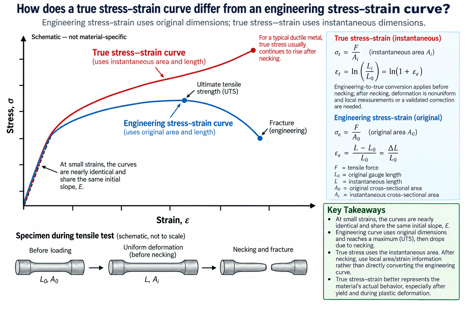
10. How does a true stress–strain curve differ from an engineering stress–strain curve?Materials And Material SelectionMedium

Short Interview Answer (30-60 seconds)

Engineering stress–strain uses the specimen's original dimensions: engineering stress is F/A0 and engineering strain is ΔL/L0. True stress–strain uses the specimen's current dimensions: true stress is F/Ai and true logarithmic strain is ln(Li/L0). At small strains, the two curves are nearly identical and have the same initial elastic slope. As plastic deformation increases, they separate. For a typical ductile metal, the engineering curve reaches ultimate tensile strength and then falls after necking, while local true stress usually continues to rise because the neck area is shrinking. After necking, deformation is nonuniform, so reliable true stress–strain data require local measurements or a validated correction rather than a simple global conversion.

Detailed Explanation

Engineering and true stress–strain curves describe the same tensile test using different reference dimensions.

Engineering stress uses the original cross-sectional area:

σe = F/A0

where F is the tensile force and A0 is the original cross-sectional area.

Engineering strain uses the original gauge length:

εe = (L - L0)/L0 = ΔL/L0

where L0 is the original gauge length and L is the current gauge length.

True stress uses the instantaneous cross-sectional area:

σt = F/Ai

where Ai is the instantaneous cross-sectional area.

True logarithmic strain is:

εt = ∫(dL/L) = ln(Li/L0)

where Li is the current gauge length. Before necking, when deformation is approximately uniform, the engineering and true strains are related by:

εt = ln(1 + εe)

At small strains, the dimensional changes are small, so engineering and true stress–strain values are nearly identical. Their initial elastic slopes are the same and correspond to Young's modulus E.

As plastic deformation increases, the specimen becomes longer and thinner. Engineering stress continues to divide the tensile force by the original area A0 even though the actual area is decreasing. True stress instead uses the current area Ai, so the true stress becomes higher than the corresponding engineering stress as the specimen thins.

For a typical ductile metal, the engineering stress–strain curve rises to the ultimate tensile strength, or UTS. Necking then begins and deformation becomes localized. The tensile force eventually decreases, and because engineering stress still divides that force by A0, the engineering stress drops toward fracture.

The local true stress in the neck behaves differently. The neck cross-sectional area decreases rapidly, and for a typical ductile metal the reduction in local area is sufficient for the local true stress to continue rising even while the tensile force falls.

The important limitation is that simple engineering-to-true conversion should not be extended blindly through necking. Before necking, deformation is approximately uniform, so global engineering measurements can be converted to true quantities using the usual relationships and the assumptions behind them. After necking, deformation is nonuniform and concentrated in the neck. Reliable post-necking true stress–strain behavior therefore requires local area and strain measurements or an appropriate validated correction method.

Useful Questions to Ask the Interviewer
  • Are we discussing only uniform deformation before necking, or should I also explain post-necking behavior?
  • Should I assume a typical ductile metal under uniaxial tension?
  • Do you want just the definitions, or also the reason the two curves diverge?
  • Should I discuss the limits of converting engineering stress–strain data into true stress–strain data after necking?

These questions matter because the interpretation changes once deformation becomes localized. Before necking, one global gauge-section description is approximately representative. After necking, the local state in the neck can differ significantly from the average gauge-section deformation.

How does a true stress–strain curve differ from an engineering stress–strain curve? diagram
How to Explain It in an Interview

I would start with the reference dimensions. Engineering stress and strain use the original specimen dimensions, while true stress and strain use the current deformation state.

Then I would define the quantities: σe = F/A0 and εe = ΔL/L0 for engineering values, compared with σt = F/Ai and εt = ln(Li/L0) for true values.

Next I would explain the curve shape. At small strain, the two descriptions are nearly the same. As plastic deformation increases and the specimen gets thinner, true stress becomes higher than engineering stress because it uses the smaller instantaneous area.

For a typical ductile metal, the engineering curve reaches UTS and then drops after necking because the load decreases while engineering stress still uses the original area. The local true stress usually continues to rise because it uses the shrinking neck area.

Finally, I would state the limitation: once necking begins, deformation is nonuniform, so I would not directly convert the global engineering curve and call the result the local true stress–strain curve. I would use local area and local strain measurements or a validated post-necking correction.

Technical Approach
  1. Identify the reference configuration used for stress and strain.
  2. Define engineering stress as σe = F/A0 and engineering strain as εe = ΔL/L0.
  3. Define true stress as σt = F/Ai and true logarithmic strain as εt = ln(Li/L0).
  4. Compare the curves at small strain, where dimensional changes are small and the curves are nearly identical.
  5. Follow the specimen into plastic deformation and recognize that its cross-sectional area decreases.
  6. Identify the engineering UTS point and the onset of necking for a typical ductile tensile specimen.
  7. Explain that engineering stress drops after necking because the tensile force decreases while A0 remains the calculation area.
  8. Explain that local true stress usually continues to rise because it uses the shrinking instantaneous neck area.
  9. Separate the uniform-deformation region from the post-necking region.
  10. For post-necking characterization, use local area and strain measurements or a validated correction rather than blindly applying a global engineering-to-true conversion.
Practical Insights

The main tradeoff is simplicity versus how closely the reported quantities follow the changing specimen geometry. Engineering stress and strain are simple because they use the original dimensions. They are useful for familiar tensile-test quantities such as yield strength and UTS. True stress and strain account for changing geometry and are more useful for describing large plastic deformation. The difficult part comes after necking, because deformation is localized and local area and strain must be measured or estimated correctly. The two curves do not represent different materials; they are different ways of describing the same tensile response.

Why Interviewers Ask This

Interviewers want to see whether you understand how the reference dimensions used in a tensile test affect the reported stress and strain, especially as plastic deformation increases and necking begins. They are also testing whether you know the limits of converting engineering stress–strain data into true stress–strain data.

Common interview mistakes

Common mistakes include using the original area in the true-stress equation; saying engineering and true curves are exactly identical throughout the elastic region instead of nearly identical at small strain; confusing stiffness with strength; assuming that true stress must fall when the tensile force falls; saying the simple relation εt = ln(1 + εe) is sufficient for local post-necking behavior; and forgetting that after necking the deformation is nonuniform, so local area and strain information or a validated correction is needed.

Interview tip

Lead with the reference dimensions: original dimensions for engineering quantities and instantaneous dimensions for true quantities. Then explain what happens during necking. A strong answer also states the limitation that simple global engineering-to-true conversion is appropriate only while deformation is sufficiently uniform; post-necking behavior requires local measurements or a validated correction.

Interviewer may ask next
When can engineering and true stress–strain values be treated as approximately the same?

They are approximately the same at small strains because the specimen dimensions have changed only slightly. The original and instantaneous areas are then close, and ln(1 + εe) is close to εe. Both curves therefore have nearly the same initial elastic response and the same initial slope, Young's modulus E. As plastic deformation increases, changing geometry becomes important and the curves separate.

What changes in the analysis once necking begins?

Once necking begins, deformation becomes localized and is no longer uniform along the gauge section. The neck area shrinks much faster than the rest of the specimen. Engineering stress normally drops because the tensile force falls while it is still divided by the original area A0. For a typical ductile metal, the local true stress usually continues to rise because it uses the shrinking instantaneous neck area. Reliable post-necking characterization therefore requires local area and strain measurements or an appropriate validated correction rather than a direct global conversion of the engineering curve.

More questions load as you scroll

Disclaimer: This interview guide is for educational and informational purposes only. It is designed to help readers prepare, but it does not guarantee any interview result, hiring decision, offer, or outcome. Interview questions, hiring criteria, and preferred answers can vary by employer, interviewer, industry, location, and time. All answers, examples, and explanations in this guide are suggested examples for interview preparation, not definitive answers or instructions for professional practice. They are based on research and judgment, are provided without warranties of any kind, and should be adapted to the question, role, and applicable laws and professional requirements. Diagrams are simplified illustrations intended to highlight the main concepts and their relationships; actual situations, systems, and practices may be more complex. Alternative approaches may be equally valid or better suited to a particular question, context, or interviewer. To the fullest extent permitted by applicable law, the contributors and publisher are not liable for decisions made, actions taken, or losses incurred based on this guide.

State Laws and Professional Responsibilities: Laws and requirements governing an occupation vary by state and jurisdiction. You are responsible for checking the current laws, licensing requirements, and scope-of-practice rules that apply to your location and role, and for ensuring that your answers and actions comply with them. Adapt examples in this guide to those requirements. This guide is not legal advice.

Content Accuracy and Verification: To the fullest extent permitted by applicable law, we do not represent or warrant that interview guides, questions, answers, examples, or diagrams are accurate, complete, current, error-free, or suitable for any particular purpose. You are responsible for independently reviewing and verifying the information before relying on it.