11 Perplexity AI Engineer Interview Questions & Answers

perplexity icon

Questions with Detailed ExplanationsWith Detailed Explanations

(Last Updated: August 28, 2026)

1. Extend the ToDo List for AI so dependent tasks stay BLOCKED until all parent tasks SUCCEED.Ai Agents And Agentic SystemsMediumPerplexity

Question Details

Accept parent task IDs during task creation; initialize a child as BLOCKED unless every parent is SUCCEEDED; after a parent succeeds, move the child to READY only when all of its parents have succeeded.

Short Interview Answer (30-60 seconds)

At a high level, I would store each task with its parent task IDs and current status. The main challenge is stopping a child from running too early. I would explain two flows: creating the task and reacting when a parent succeeds. A new dependent task starts BLOCKED, then becomes READY only if every parent is SUCCEEDED. After any parent succeeds, affected children are checked again. The trade-off is repeated checks, but the dependency rule stays simple and correct.

Detailed Explanation

The system must stop a dependent task from starting before all required parent work is finished. For example, T3 may depend on T1 and T2. T3 must stay BLOCKED while either parent is not SUCCEEDED. The important part is applying this rule when T3 is created and again when a parent later succeeds. The diagram does this with a stored Task Record, a status check, and a Parent Succeeds Event that finds affected children and checks them again.

Useful Questions to Ask the Interviewer
  1. Can a task have zero, one, or many parent task IDs?
  2. Is SUCCEEDED the only parent state that can unblock a child?
  3. Should a child become READY as soon as its last parent succeeds?
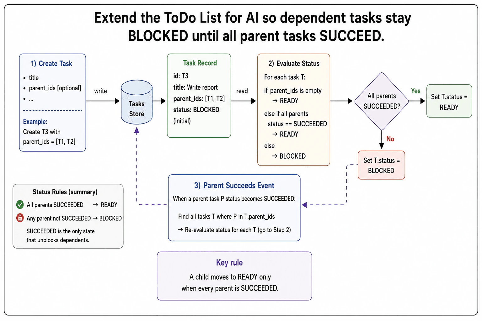
Extend the ToDo List for AI so dependent tasks stay BLOCKED until all parent tasks SUCCEED. diagram
How to Explain It in an Interview
1. Explain the main dependency rule

I would start with one simple rule: a child becomes READY only when every parent is SUCCEEDED. If even one parent has another status, the child stays BLOCKED. A task with no parents becomes READY because it has nothing to wait for.

This same rule is used during task creation and during later parent updates. That keeps the behavior easy to understand.

2. Create and store the task

For the create path, the request accepts optional parent_ids. The diagram uses T3 as an example with parents T1 and T2. The task is written to the Tasks Store, which keeps the task and its dependency information.

The Task Record contains the task ID, title, parent IDs, and status. For the dependent example, T3 starts as BLOCKED before the parent check decides whether it can move to READY.

3. Evaluate the initial status

Next, we evaluate the task status. If parent_ids is empty, the task becomes READY. If parents exist, we check their current statuses.

If every parent is SUCCEEDED, we set T.status to READY. Otherwise, we set T.status to BLOCKED. This prevents a dependent task from becoming runnable before all required work is complete.

4. Handle the Parent Succeeds Event

The second flow starts when a parent task P becomes SUCCEEDED. We find every task T whose parent_ids contains P. Those tasks are the children affected by this parent update.

Each matching child goes back through the same status evaluation. We do not make a child READY just because one parent finished. We check all of its parents again.

5. Keep the child BLOCKED until every parent succeeds

The final decision stays simple. If all parents are SUCCEEDED, the child moves to READY. If any parent is not SUCCEEDED, the child remains BLOCKED.

The benefit is one clear rule for both flows. The downside is repeated checking. A child may be evaluated several times as different parents finish, but this prevents it from running too early.

Practical Complexity & Trade-offs

The benefit is that one simple rule controls every dependency. A child becomes READY only when every parent is SUCCEEDED. The same check is used when the task is created and when a parent later succeeds. This makes the behavior easier to reason about and keeps both flows consistent. The downside is extra checking. When one parent succeeds, the system finds its dependent children and checks all parents for each child again. A child with several parents may be checked several times. We accept that extra work because it prevents dependent tasks from starting before all required parent work is complete.

Why Interviewers Ask This

The interviewer wants to see whether you can turn a dependency rule into correct state changes. They also want to see whether you notice both important moments: task creation and parent completion. A strong answer uses the same rule in both places, avoids unblocking a child too early, and explains the state flow clearly without adding unnecessary system parts.
Interviewer may ask next
What would happen if one parent finishes with FAILED instead of SUCCEEDED?

I would keep the same dependency design. The key rule still says that only SUCCEEDED parents can unblock a child. If one parent is FAILED, then the condition that all parents are SUCCEEDED is false, so the child stays BLOCKED.

The create flow works the same way. We store the child and its parent IDs, then evaluate every parent. A FAILED parent means the child cannot move to READY.

The Parent Succeeds Event also stays unchanged. It runs when a parent becomes SUCCEEDED and then checks affected children again. During that check, every parent still has to be SUCCEEDED.

The current diagram does not define a separate child state for a failed dependency. I would therefore keep the child BLOCKED rather than inventing new behavior. The downside is that the child may stay BLOCKED until another rule or user action deals with the failed parent.

What happens when a child has many parents that succeed at different times?

I would use the same status check after every parent success. Each time a parent becomes SUCCEEDED, the Parent Succeeds Event finds children that list that parent and sends those children through the status evaluation again.

Suppose T3 depends on T1, T2, and T4. If T1 succeeds first, T3 is checked but stays BLOCKED because T2 and T4 are not both SUCCEEDED. When T2 succeeds, T3 is checked again and still stays BLOCKED if T4 is unfinished. When T4 finally succeeds, the next check sees that all three parents are SUCCEEDED, so T3 moves to READY.

This keeps correctness simple because no single parent can unblock the child by itself. The downside is repeated work. The same child can be evaluated several times while different parents finish.

2. When a task FAILS, recursively mark every direct and indirect dependent task as FAILED.Ai Agents And Agentic SystemsHardPerplexity

Question Details

Propagate FAILED through the dependency graph so every direct and indirect descendant of the failed task also becomes FAILED.

Short Interview Answer (30-60 seconds)

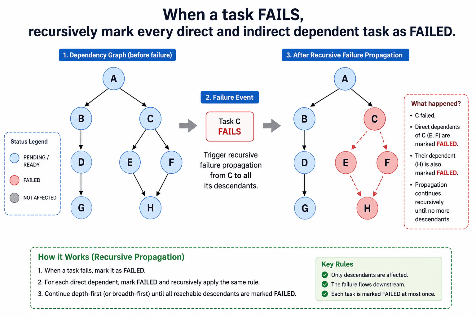
At a high level, the goal is to stop work that depends on a failed task. The main challenge is finding every downstream task, including indirect dependents. I would explain this in three steps: identify the failed task, visit each direct dependent, then continue recursively through its descendants. In the diagram, C fails, so E, F, and H also become FAILED. The trade-off is that we must traverse the dependency graph, but unaffected branches stay unchanged.

Detailed Explanation

The system must make sure a task cannot continue when something it depends on has failed. The difficult part is that the affected task may be several steps away from the original failure. For example, C fails first. E and F depend directly on C, so they fail too. H depends on E and F, so H must also fail. The other branch, B to D to G, does not depend on C and stays unchanged. The solution follows dependency arrows downstream until there are no more descendants to visit.

Useful Questions to Ask the Interviewer
  1. Can the dependency graph contain shared descendants, like H depending on both E and F?
  2. Should an already FAILED task be skipped if another path reaches it again?
  3. Can we assume the dependency graph has no cycles?
When a task FAILS, recursively mark every direct and indirect dependent task as FAILED. diagram
How to Explain It in an Interview
1. Start with the dependency direction

I would first make the arrow meaning clear. An arrow points from one task to another task that depends on it. In the diagram, C points to E and F. That means E and F depend on C. If C fails, both must become FAILED. This direction matters because failure moves only toward descendants, not toward tasks above C.

2. Mark the original failed task

When C fails, I mark C as FAILED. This is the starting failure shown in the diagram. I do not change A, B, D, or G because they are not descendants of C. This keeps the update limited to tasks that actually depend on the failed work.

3. Visit every direct dependent

Next, I look at the tasks that depend directly on C. Those tasks are E and F. I mark both as FAILED. Then I apply the same rule to each of them. This repeated step is recursion. In simple words, the same failure rule is applied again to each dependent task.

4. Continue through indirect descendants

E and F both lead to H. H does not depend directly on C, but it is still a descendant of C. Therefore H must also become FAILED. A depth-first or breadth-first walk can find every reachable descendant. Either approach works here. The important rule is to keep following dependency arrows until no new descendant remains.

5. Leave unrelated tasks unchanged

The B to D to G branch stays unchanged. None of those tasks depends on C. This matters because a failure should not spread into unrelated work. H can be reached through both E and F, so it should be marked FAILED only once. A visited check, or an equivalent already-FAILED check, prevents repeated work. The benefit is correct failure handling. The downside is that the system must walk the affected part of the graph whenever a task fails.

Practical Complexity & Trade-offs

The benefit is that every task depending on failed work is stopped correctly. Unrelated tasks keep their current state, so one failure does not cancel the whole graph. The downside is that the system must visit the affected descendants. If many tasks depend on one failed task, this walk can touch many tasks and dependency edges. A visited check also matters when two paths reach the same task, such as H through E and F. This prevents repeated work. Depth-first and breadth-first search both work because the goal is simply to reach every downstream descendant.

Why Interviewers Ask This

Interviewers use this question to test whether you understand dependency graphs and failure handling. They want to see if you follow arrows in the correct direction and include indirect dependents, not only direct ones. They also look for careful handling of shared descendants so the same task is not processed repeatedly. A strong answer shows that you can turn a simple rule into a correct graph traversal.

Interviewer may ask next
What changes if the same dependent task can be reached through several dependency paths?

I would keep the same failure flow, but I would track which tasks were already visited. In the diagram, H can be reached through both E and F. Without a visited check, the traversal could try to process H twice. The first time H is reached, I mark it FAILED and record that it has been visited. If another path reaches H later, I skip it because its state is already correct. This does not change which tasks fail. C, E, F, and H still become FAILED, while A, B, D, and G stay unchanged. The visited check only prevents repeated work. It also makes the logic safer for larger graphs with many shared descendants. The downside is a small amount of extra memory because the traversal must remember which tasks it has already processed.

What would you do if the dependency graph could contain a cycle?

I would still follow the same downstream failure rule, but a visited check would become required. A cycle means following dependency arrows could eventually return to a task already seen. Without protection, a recursive walk could continue forever. I would mark the current task FAILED, record it as visited, and then examine its dependents. Before visiting a dependent, I would check whether that task was already visited. If it was, I would skip it. The result stays the same: every reachable task from the original failure becomes FAILED, and unrelated tasks stay unchanged. This keeps the traversal correct even when the graph contains a cycle. The main downside is that the traversal needs extra memory for visited tasks, but that memory is needed to guarantee the walk stops.

3. Train a binary classifier on the provided toy dataset using Python and scikit-learn.Fine Tuning And Model AdaptationMediumPerplexity

Question Details

Use the predetermined toy dataset, choose and fit an appropriate scikit-learn binary classifier, and report its initial evaluation result.

Short Interview Answer (30-60 seconds)

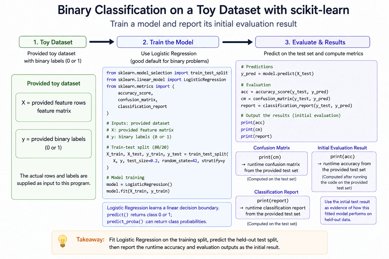
I would use Logistic Regression as a simple binary classifier. I would split the provided X and y into training and test data, fit the model on the training part, predict the test part, and report the runtime accuracy, confusion matrix, and classification report. The important point is that I would report the values produced from the provided data instead of assuming a score in advance.

Detailed Explanation

See the Code while reading this explanation.

The task is to teach a program to choose between two possible labels using examples that already have the correct answer. I would keep most examples for learning and save some examples for checking the result. The program learns from the first group and then makes choices for the saved group. I would compare those choices with the real answers and report what happened. I would not make up a score because the real result depends on the supplied rows and labels.

Useful Questions to Ask the Interviewer
  1. Are X and y already provided as Python objects?
  2. Should I use the requested split settings exactly, including 20 percent for testing and stratification?
  3. Do you want only accuracy, or should I also show the confusion matrix and classification report?
Train a binary classifier on the provided toy dataset using Python and scikit-learn. diagram
How to Explain It in an Interview

I would start with the provided feature matrix X and binary labels y. A binary label means each example belongs to one of two classes, such as 0 or 1.

I would use Logistic Regression. It is a simple supervised classifier that learns a linear decision boundary from labeled training examples. I would split the supplied data so that 80 percent is used for training and 20 percent is kept for testing. I would use random_state equal to 42 so the split can be repeated. I would also use stratify equal to y so the split tries to keep the class proportions similar in both parts.

Next, I would call fit on X_train and y_train. This is the training step. The model learns parameters from those labeled examples. I would then call predict on X_test. The predict method returns class 0 or class 1. If I needed class probabilities, I could use predict_proba instead.

For the initial evaluation, I would calculate accuracy, a confusion matrix, and a classification report. Accuracy shows the fraction of test predictions that are correct. The confusion matrix shows how predictions are distributed across the two true classes. The classification report gives measures such as precision and recall for each class.

The exact result must come from running the code on the provided dataset. The supplied prompt does not include the actual toy rows, so a numeric result is not supported here. I would report the runtime values produced by print(acc), print(cm), and print(report). One limitation is that a small test set can give an unstable estimate. Stratification can also fail when a class has too few examples. In production, I would use a stronger validation process before treating this initial result as reliable evidence.

Key Insight / Why This Solution Works
  1. Use the supplied X feature matrix and y binary labels.
  2. Split the data into training and test parts with test_size equal to 0.2, random_state equal to 42, and stratify equal to y.
  3. Create a LogisticRegression classifier.
  4. Fit the classifier with X_train and y_train.
  5. Predict labels for X_test with predict.
  6. Compute accuracy_score, confusion_matrix, and classification_report from y_test and the predictions.
  7. Print and report the runtime results. This task uses standard supervised classifier training. Prompting, retrieval, preference tuning, and language model fine tuning are not needed for this toy classifier.
Code
import json
import sys

from sklearn.linear_model import LogisticRegression
from sklearn.metrics import accuracy_score, classification_report, confusion_matrix
from sklearn.model_selection import train_test_split


def main() -> None:
    # Read the provided feature rows and labels without inventing toy data.
    payload = json.load(sys.stdin)
    X = payload["X"]
    y = payload["y"]

    # Keep 20 percent of the provided data for an unseen test check.
    X_train, X_test, y_train, y_test = train_test_split(
        X,
        y,
        test_size=0.2,
        random_state=42,
        stratify=y,
    )

    # Fit the binary classifier only on the training part.
    model = LogisticRegression()
    model.fit(X_train, y_train)

    # Predict class labels for the held out test examples.
    y_pred = model.predict(X_test)

    # Compute the same initial evaluation outputs shown in the diagram.
    acc = accuracy_score(y_test, y_pred)
    cm = confusion_matrix(y_test, y_pred)
    report = classification_report(y_test, y_pred)

    print(acc)
    print(cm)
    print(report)


if __name__ == "__main__":
    main()
Why Interviewers Ask This

Interviewers ask this question to check whether I can turn labeled data into a simple supervised learning workflow. They want to see that I separate training data from test data, fit an appropriate classifier, make predictions on unseen examples, and measure the result correctly. They also want to see that I do not invent evaluation numbers before the code is run on the provided data.

Common interview mistakes

A common mistake is training and testing on the same rows. That gives an overly optimistic result because the model is checked on data it already saw. Another mistake is inventing an accuracy value before running the provided dataset. It is also incorrect to say that predict directly returns probabilities. Predict returns class labels, while predict_proba can return class probabilities. A candidate should also remember that stratified splitting needs enough examples from each class. Finally, using only accuracy can hide class specific errors, so the confusion matrix and classification report give useful extra evidence.

Interview tip

Explain the flow in order: provided data, split, fit, predict, then evaluate. State clearly that the final numbers must come from running the supplied dataset. Also distinguish predict, which returns class labels, from predict_proba, which can return probabilities.

Interviewer may ask next
What happens if one class has too few examples for the stratified split?

The stratified split can fail because it needs enough examples from each class to place class members into both parts. I would first inspect the class counts. For a very small toy dataset, I might need a different split strategy or more examples. This matters because removing stratification can make the test set less representative, while keeping stratification is impossible when a class does not have enough samples.

Why use Logistic Regression here instead of a more complex classifier?

Logistic Regression is a good first choice because it is simple, fast, and suitable for binary classification. It gives a clear baseline before adding model complexity. If the data pattern is not well represented by a linear decision boundary, a more flexible classifier may perform better. The tradeoff is that more flexible models can add tuning cost, harder interpretation, and greater risk of fitting noise on a small toy dataset.

4. Improve the binary classifier's initial evaluation metric through model choice or tuning.Fine Tuning And Model AdaptationHardPerplexity

Question Details

Starting from the initial classifier, make a defensible model-selection or tuning change and compare the resulting metric with the original baseline on the same provided task.

Short Interview Answer (30-60 seconds)

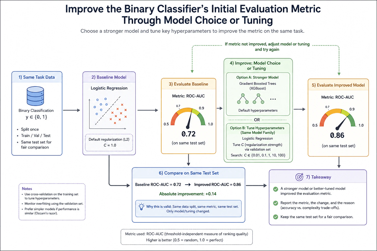
I would keep the same task, data split, and ROC AUC metric, then make one defensible change and measure whether it helps. The baseline is logistic regression with ROC AUC of 0.72. I can try Gradient Boosted Trees with XGBoost, or keep logistic regression and tune its regularization value C using validation data. I would choose the best validated option, then evaluate it on the same test set. In the diagram, the improved ROC AUC is 0.86, so the absolute improvement is 0.14.

Detailed Explanation

The goal is to improve the classifier without making the comparison unfair. I keep the same binary classification task, the same train, validation, and test split, and the same ROC AUC metric. The baseline is logistic regression with ROC AUC of 0.72. I then change only the model choice or its tuning. I can try Gradient Boosted Trees with XGBoost, or tune the logistic regression regularization value C. I use validation data to make that choice. Finally, I evaluate the selected model on the same test set and compare the result with the baseline.

Useful Questions to Ask the Interviewer
  1. Should ROC AUC remain the main metric for the comparison?
  2. Is the test set fixed and untouched until the final evaluation?
  3. May I change the model family, or should I tune only the original logistic regression model?
Improve the binary classifier's initial evaluation metric through model choice or tuning. diagram
How to Explain It in an Interview

I would start with the baseline shown in the diagram. The model is logistic regression with L2 regularization and C equal to 1.0. Its ROC AUC is 0.72 on the test set.

Next, I would make one controlled change. One option is Gradient Boosted Trees with XGBoost. The diagram shows this as a stronger model choice using its default settings. Another option is to keep logistic regression and tune C, which controls the strength of regularization. The candidate values shown are 0.01, 0.1, 1, 10, and 100.

I would use the validation set to compare choices. If I need a more stable tuning estimate, I can use cross validation on the training data. I would not repeatedly use the test score while selecting the model or C value. Doing that would let test information influence the choice and make the final result less trustworthy.

After selection, I would evaluate the chosen model on the same test set with the same ROC AUC metric. The diagram shows the improved model reaching 0.86. Compared with the baseline of 0.72, the absolute improvement is 0.14.

If the metric does not improve, I would change the model choice or tuning and repeat the validation step. I would also watch for overfitting. If a simpler model gives nearly the same result, I would usually prefer it because it is easier to operate and explain.

Technical Approach
  1. Keep the same binary classification task, data split, and ROC AUC metric.
  2. Measure the logistic regression baseline. The diagram shows ROC AUC of 0.72.
  3. Make one controlled adaptation choice. Try Gradient Boosted Trees with XGBoost, or keep logistic regression and tune C.
  4. If tuning C, compare values such as 0.01, 0.1, 1, 10, and 100 using validation data. Cross validation can be run on the training data for a more stable choice.
  5. Select the best validated option while watching for overfitting.
  6. Evaluate that selected model on the same untouched test set.
  7. Compare the final ROC AUC with the baseline. The diagram shows 0.86 versus 0.72, which is an absolute improvement of 0.14.
  8. If the metric does not improve, revise the model choice or tuning and repeat the validation process without tuning against the test set.
Why Interviewers Ask This

The interviewer wants to see whether I can improve a classifier while keeping the comparison fair. I should know how to hold the task, data split, and evaluation metric constant while changing the model choice or tuning. They also want to see whether I understand validation, cross validation, overfitting, test set isolation, and the tradeoff between better performance and added model complexity.

Common interview mistakes

A common mistake is choosing hyperparameters by repeatedly checking the test score. That allows test information to affect model selection and makes the final comparison less trustworthy. Another mistake is comparing models on different data splits or with different metrics. A candidate may also assume that a more complex model must be better. The stronger model should justify its added complexity with better validated performance. Another mistake is ignoring overfitting when the validation result improves but the final test result does not.

Interview tip

State the fairness rule first: same task, same data split, and same ROC AUC metric. Then explain exactly one model or tuning change, how validation selects it, and why the test set stays outside that selection loop. Finish with the diagram result: ROC AUC improves from 0.72 to 0.86, which is an absolute gain of 0.14.

Interviewer may ask next
What would you do if validation ROC AUC improves but test ROC AUC does not?

I would not accept the new model as a proven improvement. That result means the validation gain did not carry over to the untouched test set. I would check for overfitting, unstable validation results, data leakage, and differences between the validation and test data. I would then revise the model choice or tuning using only training and validation data. The key tradeoff is that more tuning can fit noise, so the test set must remain outside the selection loop.

When would you tune logistic regression instead of moving to Gradient Boosted Trees?

I would tune logistic regression when the simpler model is already close to the required quality or when simplicity, speed, and easier operation matter. I would tune C using validation data and compare the result with the same baseline. Gradient Boosted Trees can represent more complex patterns, but they add model complexity. The decision depends on whether the ROC AUC gain is large enough to justify that extra complexity while keeping the evaluation process unchanged.

5. Design a system for detecting and ranking trending queries.Ai System DesignMediumPerplexity

Question Details

Cover real-time query-event ingestion, streaming aggregation, trend scoring and ranking, low-latency serving, personalization, and abuse mitigation.

Short Interview Answer (30-60 seconds)

At a high level, I would build a streaming system that finds queries whose interest is rising compared with a recent baseline. Query events first pass through an ingestion gateway, then a partitioned event stream. Stream processors normalize queries, count them in sliding windows, and create trend features. A scoring service ranks the strongest trends and stores Top-K results for fast serving. The serving API can personalize results using user signals. Abuse controls reduce gaming. The main trade-off is freshness versus processing, storage, and ranking cost.

Detailed Explanation

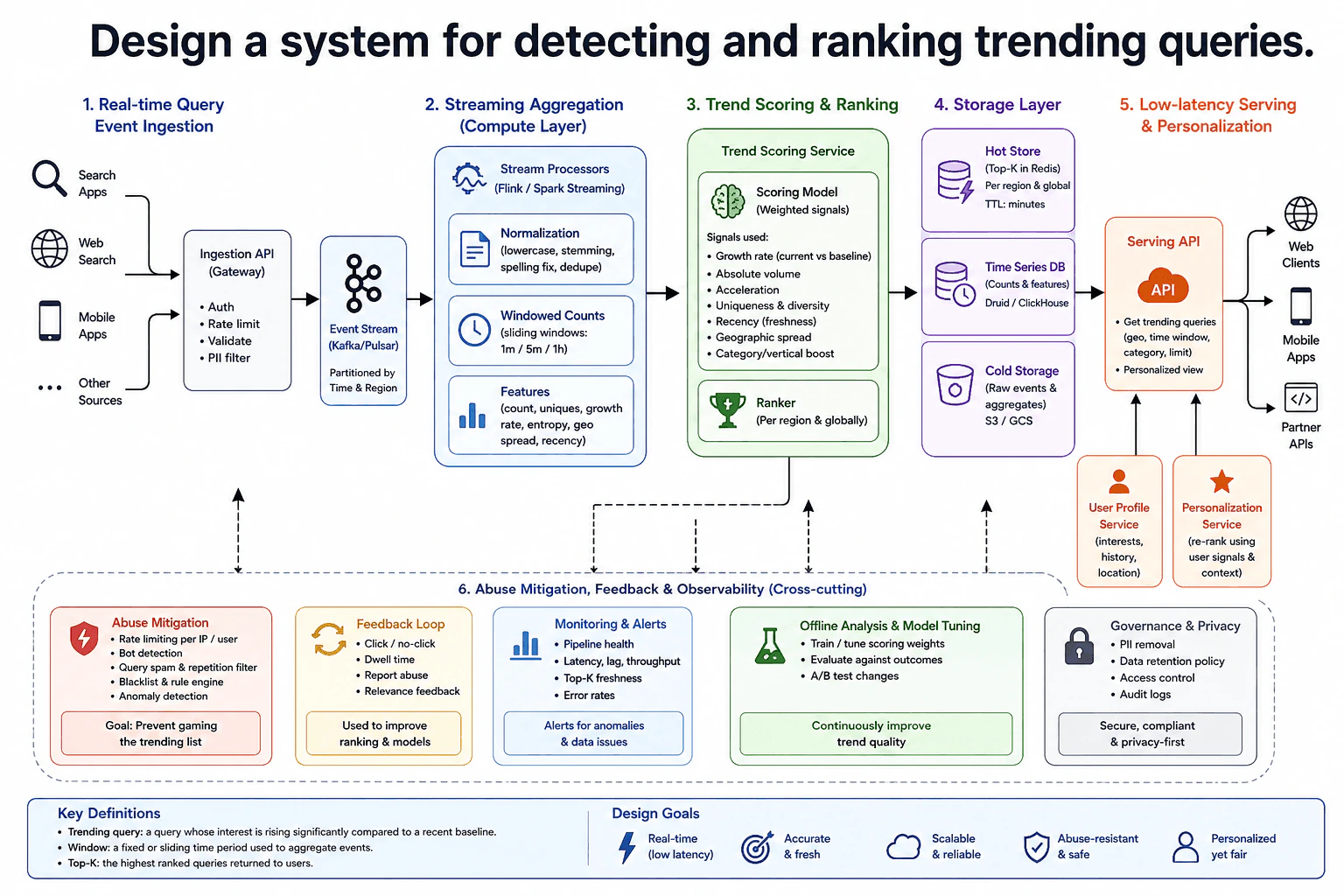
This system finds search queries that are becoming popular right now. For example, a query may suddenly get much more interest than it had a few minutes ago. We need to notice that change quickly, rank the strongest trends, and return them with low delay. The hard part is separating real interest from normal traffic, spam, and fake bursts. The design also needs regional and personalized results. I would follow the diagram from query collection, through counting and scoring, and finally to serving, feedback, and monitoring.

Useful Questions to Ask the Interviewer
  • How fresh should the trending list feel to users?
  • Do we need global trends, regional trends, or both?
  • How much personalization should change the public trending list?
  • Which kinds of abusive traffic should we block or reduce?
Design a system for detecting and ranking trending queries. diagram
How to Explain It in an Interview
1. Collect and validate query events

I would start with the real-time query events. Search Apps, Web Search, Mobile Apps, and Other Sources send events to the Ingestion API Gateway. The gateway handles authentication, rate limiting, validation, and PII filtering. PII means personal information that should not enter the trend pipeline unnecessarily. These checks matter because invalid, abusive, or sensitive events should be handled before aggregation. Valid events then move into the Event Stream. The diagram uses Kafka or Pulsar. The stream is shown as partitioned by time and region so processing can be divided across groups of events.

2. Normalize queries and aggregate recent activity

Stream Processors, shown as Flink or Spark Streaming, consume the Event Stream. They first normalize query text. The diagram shows lowercasing, stemming, spelling fixes, and deduplication. The goal is to avoid treating small text differences as unrelated trends. The processors then keep sliding windows such as 1 minute, 5 minutes, and 1 hour. A sliding window is a recent time range that keeps moving forward. For each query, the system creates features such as counts, unique activity, growth rate, entropy, geographic spread, and recency. These features become inputs to trend scoring.

3. Score and rank trending candidates

The Trend Scoring Service turns those features into a trend score. The Scoring Model uses weighted signals shown in the diagram. These include growth rate versus a baseline, absolute volume, acceleration, uniqueness and diversity, recency, geographic spread, and category or vertical boosts. Growth helps detect rising interest. Absolute volume helps avoid overvaluing tiny changes. Recency favors fresh activity. The Ranker then orders candidates per region and globally. This produces the Top-K queries, meaning the highest-ranked queries are kept for fast serving.

4. Store hot results and historical data

The Storage Layer has three jobs. The Hot Store keeps Top-K results in Redis for each region and globally. Its time-to-live is measured in minutes, so old results can expire. The Time Series DB, shown as Druid or ClickHouse, stores counts and features over time. This supports comparisons between current and earlier behavior. Cold Storage, shown as S3 or GCS, keeps raw events and aggregates for longer-term analysis. These stores serve different needs. Redis supports fast reads, while the other stores support historical analysis and tuning.

5. Serve and personalize the trending list

The Serving API gets prepared trend data from the Storage Layer and returns results to Web Clients, Mobile Apps, and Partner APIs. The diagram shows inputs such as geography, time window, category, and result limit. The API can also return a personalized view. The User Profile Service supplies interests, history, and location. The Personalization Service re-ranks the existing trend candidates using user signals and context. This keeps the main trend-detection logic separate from user-specific ordering.

6. Protect quality and improve the system

Abuse Mitigation works across the design. It includes per-IP or per-user rate limiting, bot detection, query spam and repetition filters, blacklist rules, and anomaly detection. Its goal is to prevent people or automated systems from gaming the trending list. The Feedback Loop collects click or no-click signals, dwell time, abuse reports, and relevance feedback. Offline Analysis and Model Tuning use historical outcomes to improve scoring weights, evaluate against outcomes, and test changes. Monitoring and Alerts watch pipeline health, latency, lag, throughput, Top-K freshness, and error rates. Governance and Privacy add PII removal, data retention rules, access control, and audit logs. These supporting flows improve quality and safety without becoming the client response path.

Practical Complexity & Trade-offs

The main trade-off is freshness versus cost and stability. Short sliding windows notice new trends quickly, but they can react strongly to noise and sudden bursts. Longer windows are steadier, but they respond more slowly. Keeping Top-K results in Redis makes serving fast, but complete history must live elsewhere. Regional ranking gives more useful local trends, but it increases processing and storage work. Personalization can improve relevance, but it needs user signals and careful privacy controls. Abuse filters reduce manipulation, but aggressive filters can also suppress real breaking events. We accept these costs because a useful trending system must stay fresh, fast, scalable, hard to game, and practical to operate.

Why Interviewers Ask This

Interviewers use this question to test whether a candidate can design a real-time data system from end to end. They want clear thinking about streaming, time windows, feature creation, ranking, storage, and fast serving. They also look for judgment around personalization, privacy, abuse, feedback, and monitoring. A strong answer explains why each component exists and clearly discusses the trade-offs between freshness, ranking quality, scalability, and operational cost.

Interviewer may ask next
How would you handle a sudden traffic spike during a major breaking event?

I would keep the same architecture and increase capacity around the Event Stream and Stream Processors. The event stream is already divided into partitions, so processing work can be spread across more workers as traffic grows. I would watch pipeline lag, throughput, latency, and Top-K freshness through Monitoring and Alerts. Those signals show whether aggregation is falling behind. The scoring rules should remain consistent so extra traffic does not change what the trend score means. The Serving API can continue reading prepared Top-K results from the Hot Store, which separates low-latency reads from heavier streaming work. Abuse Mitigation also remains important because a real breaking event can attract bots and repeated queries. The main downside is higher compute and streaming cost during the spike. More processing capacity also increases operational complexity. I would accept that cost because the system needs to preserve fresh rankings while large volumes move through the pipeline.

How would you stop bots from pushing a fake query into the trending list?

I would use the Abuse Mitigation controls already shown in the design. The Ingestion API Gateway applies rate limits and validates incoming events. The abuse layer then looks for bots, repeated queries, query spam, blacklist matches, and anomalous patterns. These controls can remove or reduce suspicious activity before it has too much influence on ranking. The Trend Scoring Service also uses more than raw volume. It considers growth, uniqueness and diversity, geographic spread, recency, acceleration, and other signals. That makes a simple repeated burst less convincing than broad activity from many users and locations. Abuse reports from the Feedback Loop provide another signal for later analysis. Monitoring can alert operators when unusual patterns appear. The main downside is false positives. A real breaking event can also create a sudden burst. For that reason, I would combine several signals instead of treating high volume alone as proof of manipulation.

6. Design a search system that adapts to constantly changing user interests.NEWAi System DesignHardPerplexity

Question Details

Design an end-to-end personalized search system that responds to both the current query and changing user interests. Cover interaction-event ingestion, session and long-term interest representations, candidate retrieval, ranking or reranking with recency weighting, near-real-time profile updates, cold-start behavior, exploration and diversity, privacy and deletion controls, latency and scale tradeoffs, and offline plus online evaluation for relevance and interest-drift response time.

Short Interview Answer (30-60 seconds)

At a high level, I would build a search system that learns from user behavior and adapts in near real time. Interaction events flow through Kafka or PubSub, then Flink or Spark Streaming updates short-term and long-term interest profiles. A query is understood, then BM25, vector search, personalization, and content filters retrieve candidates. Learning-to-rank uses relevance, recency, personal fit, diversity, novelty, and quality signals. I would add privacy controls, cold-start handling, caching, scaling, and evaluation. The main trade-off is faster adaptation versus latency, cost, and operational complexity.

Detailed Explanation

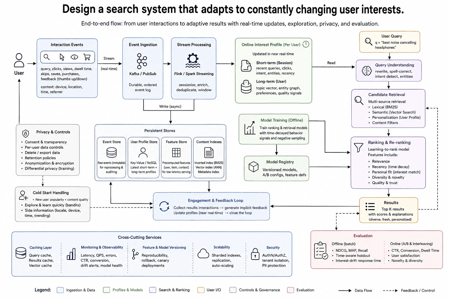
The problem is to make search follow what a person wants now, while still remembering useful older interests. A user may usually read programming content but spend today researching headphones. Search should react quickly without forgetting the longer history. It should also stay fast, work for new users, protect personal data, and avoid repetitive results. I would explain the design from user events, to profile updates, to retrieval and ranking, then close the loop with feedback and evaluation.

Useful Questions to Ask the Interviewer
  • How quickly should new behavior change search results?
  • What traffic and latency targets matter most?
  • Which user events may we store, and for how long?
  • How much exploration is acceptable compared with immediate relevance?
Design a search system that adapts to constantly changing user interests. diagram
How to Explain It in an Interview
1. Capture and process interaction events

I would start with user behavior. The system records queries, clicks, views, dwell time, skips, saves, purchases, feedback, and useful context. Event Ingestion uses Kafka or PubSub as a durable, ordered event log. Stream Processing uses Flink or Spark Streaming to sessionize, enrich, deduplicate, and window events. Processed events also write asynchronously into Persistent Stores for later use.

2. Maintain changing user interests

The Online Interest Profile has short-term and long-term parts. Short-term session interest keeps recent queries, clicks, intent, entities, and recency. Long-term interest keeps topic vectors, an entity graph, preferences, and quality signals. Stream Processing updates this profile in near real time.

Persistent Stores support this flow. The Event Store keeps raw immutable events. The User Profile Store keeps the latest profiles. The Feature Store keeps precomputed user, item, and context features. Content Indexes hold BM25, ANN vector, and metadata indexes.

3. Understand the query and retrieve candidates

The User Query goes first to Query Understanding. It can rewrite the query, correct spelling, detect intent, and identify entities. It also reads the Online Interest Profile.

Candidate Retrieval then combines lexical BM25, semantic vector search, personalization from the User Profile, and content filters. For a new user, Cold Start Handling begins with popularity and content quality. It can also use allowed side information and bandit-style exploration to learn faster.

4. Rank, diversify, and return results

Ranking and Re-ranking use a learning-to-rank model. Features include relevance, recency with time decay, personal fit, diversity, novelty, and quality or trust. Recency helps recent behavior matter more when interests shift. Diversity avoids many nearly identical results.

Offline Model Training learns ranking and retrieval models from time-decayed behavior signals and negative sampling. The Model Registry keeps versioned models, A/B configurations, and feature definitions. Results return the top K items with scores and explanations.

5. Close the feedback loop

The Engagement and Feedback Loop collects result interactions and turns them into implicit feedback. It updates profiles in near real time, so the next search can reflect the newest behavior.

Cross-cutting services keep the system practical. Query, result, and vector caches lower latency. Sharded indexes, replication, and auto-scaling support growth. Monitoring tracks latency, QPS, errors, CTR, conversion, drift alerts, and model health. Feature and model versioning supports reproducibility, rollback, and canary deployments. Security covers authentication, authorization, tenant isolation, and PII protection.

Privacy and Controls add consent, transparency, per-user controls, delete or export actions, retention policies, anonymization, encryption, and differential privacy for training. Offline evaluation uses nDCG, MAP, Recall, time-aware holdouts, and interest-drift response time. Online evaluation uses A/B testing or interleaving with CTR, conversion, dwell time, satisfaction, novelty, and diversity.

Practical Complexity & Trade-offs

The main design choice is freshness versus cost. Near-real-time profile updates make search react faster, but they require more streaming work and more serving capacity. Caching lowers latency, but stale cached results or vectors can slow adaptation. Combining BM25 and vector search improves candidate coverage, but it costs more than one retrieval method. Personalization can improve usefulness, but it also raises privacy risk. Consent, deletion controls, encryption, tenant isolation, and PII protection reduce that risk. Exploration helps discover new interests, but too much exploration can hurt immediate relevance. Sharding, replication, and auto-scaling improve scale and availability, but they add operational work. We accept these costs because fast interest adaptation is the core goal.

Why Interviewers Ask This

This question tests whether a candidate can connect streaming data, user profiles, retrieval, ranking, privacy, scaling, and evaluation into one clear system. The interviewer wants judgment about short-term versus long-term interests, recency, cold start, exploration, and diversity. They also look for practical thinking about latency, feedback loops, data protection, model updates, observability, and measurable success. A strong answer explains how the pieces work together and communicates the trade-offs clearly.

Interviewer may ask next
What would you change if user interests started changing within only a few minutes?

I would keep the same architecture, but make the short-term session profile influence ranking more strongly. Stream Processing already receives recent events through Kafka or PubSub, so I would make recent queries, clicks, dwell time, skips, and feedback update the Online Interest Profile quickly. Ranking and Re-ranking would place more weight on recency with time decay. Older behavior would still remain in the long-term profile, which helps prevent one unusual action from completely changing the user model.

I would also watch the offline interest-drift response-time metric and verify the change online with A/B testing or interleaving. Caching needs care because stale query, result, or vector caches can hide a recent interest change. Persistent Stores, Candidate Retrieval, Model Registry, privacy controls, and security stay the same.

The downside is higher streaming and serving cost. More frequent updates create more writes and more feature refreshes. The benefit is that search reacts much faster when the user's intent changes.

How would you handle a completely new user with no interaction history?

I would use the Cold Start Handling path already shown in the design. With no history, Candidate Retrieval cannot depend much on personalization yet. It can start with lexical BM25, semantic vector search, popularity, and content-quality signals. The system can also use allowed side information such as locale, device, time, or trending content. Bandit-style exploration can mix in diverse choices so the system learns the user's interests faster.

As the user clicks, skips, saves, purchases, or gives feedback, those events enter Event Ingestion and Stream Processing. The Engagement and Feedback Loop converts later result interactions into implicit feedback. The Online Interest Profile then starts building short-term and long-term signals, so future searches become more personalized.

Privacy and per-user controls stay active from the first interaction. The downside is weaker personalization at the beginning. Too much exploration can also reduce immediate relevance, so online evaluation should watch satisfaction, CTR, dwell time, novelty, and diversity.

7. How would you determine the right criteria for when to forget outdated data, update the model, and evaluate performance?Llmops And Production AiHardPerplexity

Question Details

Define a versioned lifecycle policy for user signals, retrieved knowledge, training data, and model releases. Explain how age, relevance decay, legal retention, user deletion, data drift, quality regression, and minimum evidence trigger expiration, re-indexing, retraining, fine-tuning, or no change. Include offline evaluation, shadow or canary testing, release thresholds, rollback criteria, monitoring by important data slices, and safeguards against forgetting still-valid knowledge or learning from noisy recent behavior.

Short Interview Answer (30-60 seconds)

I would use a versioned lifecycle policy. Age alone would not decide anything. I would combine relevance, legal retention, user deletion, drift, quality regression, and minimum evidence, then choose keep, expire, re-index, fine-tune, or retrain. Every model change would pass offline tests, gradual release, monitoring, and rollback gates.

Detailed Explanation

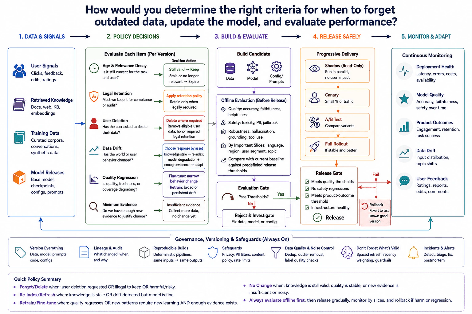
I would not remove information or change the system just because time has passed. First, I would identify what information and system versions are involved and what changed. Then I would collect evidence. I would ask whether the information is still useful, whether a law requires us to keep it, whether a user asked us to remove it, and whether recent behavior is trustworthy. I would also check whether results are getting worse. The goal is to make the smallest safe change and test it carefully before it reaches everyone.

Useful Questions to Ask the Interviewer
  1. Which assets are in scope: user signals, retrieved knowledge, training data, model versions, prompts, and configurations?
  2. What legal retention or user-deletion rules must the lifecycle policy follow?
  3. Which quality, safety, product, and infrastructure measures are release gates?
  4. Which user, language, region, topic, or other data slices are important enough to monitor separately?
  5. How much reliable new evidence is required before we allow fine-tuning or retraining?
  6. What rollback conditions and previous known-good version are available?
How would you determine the right criteria for when to forget outdated data, update the model, and evaluate performance? diagram
How to Explain It in an Interview

I would start by defining the scope and version lineage. Every important dataset, retrieved-knowledge index, model, prompt, and configuration should have a version. Lineage means I can trace which exact inputs created a model or release. I would also keep timestamps and evaluation results when they matter. This makes builds reproducible and gives me a known-good rollback point.

Next, I would collect evidence before changing anything. I would look at age, relevance, legal rules, user-deletion requests, data drift, quality regression, and the amount of reliable new evidence. The smallest useful first step is to identify which asset is actually stale or failing instead of assuming the model needs retraining.

For age and relevance decay, I would ask whether the information is still useful for the task and user. Old does not automatically mean wrong. If knowledge is still valid, I keep it. If it is stale or no longer relevant, I expire it. This protects long-lived knowledge from being forgotten too early.

For legal retention, I would apply the retention policy. Some records may have to stay for compliance or audit reasons. I would retain them only when required rather than using one unconditional keep rule.

For user deletion, I would remove eligible user data where the policy and system require it while honoring any required legal retention. I would not claim that one deletion request automatically erases information from every historical model artifact. The exact action depends on where the data exists and what the policy requires.

For retrieved knowledge, I would usually refresh the retrieval layer before changing the model. If documents, metadata, embeddings, or the index are stale, I can re-chunk, re-embed, and re-index the current knowledge. This is usually a smaller and safer change than retraining the model to learn changing facts.

For data drift, I would choose the response by asset. Data drift means the incoming data or user behavior has changed. If retrieved knowledge is stale, I refresh the index. If the model's quality is degrading and I have enough trustworthy evidence, I consider adapting the model. Drift by itself is not enough reason to retrain.

For quality regression, I would check whether required quality measures such as accuracy, faithfulness, helpfulness, or safety are getting worse. A narrow, validated behavior change may justify fine-tuning. Fine-tuning means adapting an existing model with a smaller targeted training run. A broad or persistent change in what the model needs to learn may justify retraining. I would require enough reliable evidence before either action.

Minimum evidence protects the system from noisy recent behavior. One unusual day, a small user group, duplicate events, or poor labels should not trigger a model update. I would check duplicates, outliers, label quality, and whether the pattern persists across important slices. I can also use recency weighting and guardrails. If the evidence is weak or unstable, I collect more data and make no change yet.

When a model change is justified, I build a versioned candidate from reproducible data, model, prompt, and configuration inputs. Then I run offline evaluation before any production release. Offline evaluation means testing the candidate on controlled evaluation data without exposing users to it. I compare the candidate with the current baseline against predefined release thresholds.

I would evaluate model quality such as accuracy, faithfulness, and helpfulness; safety risks such as harmful output or personal-data leakage; robustness; and important data slices such as language, region, user segment, or topic. Slice evaluation matters because a good overall average can hide a serious regression for one group.

If the candidate fails an offline threshold, I reject it and investigate the responsible data, model, prompt, or configuration. I do not release it just because one average metric improved.

If it passes offline evaluation, I move to progressive delivery. Shadow testing runs real production inputs through the candidate without letting its output affect users. This gives production-like evidence with no user impact from the candidate output. A canary release then sends only a small share of live traffic to the candidate. An A/B test can compare variants when product outcomes are part of the decision.

I move to full rollout only when the predefined release gates pass. I keep separate gates for model quality, safety, product outcomes, and infrastructure health. A service can be available and fast while its answers are worse, so deployment health and model quality must not be treated as the same thing.

After release, I monitor continuously. Deployment health includes latency, errors, cost, and availability. Model quality includes measures such as accuracy, faithfulness, and safety. Product outcomes include task success, engagement, or other outcomes that the product actually defines. I also watch data drift and user feedback. I break these measures down by important slices so a global average does not hide a local problem.

Rollback criteria are defined before release. If a critical quality, safety, product, or infrastructure threshold is broken, I revert to the last known-good version. The rollback should restore the model, prompt, configuration, and other release artifacts needed to reproduce that known-good state.

Monitoring then feeds the next lifecycle decision. The main tradeoff is stability versus freshness. Updating too slowly leaves stale knowledge or degraded behavior in production. Updating too quickly can make the system learn from noise, remove still-valid knowledge, or introduce regressions. So I prefer the smallest safe action supported by enough evidence: keep valid knowledge, expire stale information, refresh stale retrieval data, fine-tune narrow validated behavior changes, retrain broad persistent changes, or make no change when the evidence is insufficient or noisy.

Release Lifecycle
  1. Define the scope and version user-signal data, retrieved knowledge, training data, models, prompts, and configurations. Record lineage so each release can be reproduced.
  2. Collect evidence before changing anything. Check age, relevance, legal retention, user deletion, data drift, quality regression, and minimum reliable evidence.
  3. Identify the affected asset and choose the smallest justified action. Keep still-valid information. Expire stale or irrelevant information. Apply legal retention rules. Delete eligible user data where required. Re-index stale retrieved knowledge. Fine-tune narrow validated behavior changes. Retrain only for broad or persistent change with enough evidence.
  4. Build a reproducible, versioned candidate when a model or configuration change is needed.
  5. Run offline evaluation. Compare the candidate with the current baseline against predefined quality, safety, robustness, important-slice, product, and infrastructure thresholds that apply to the release.
  6. If offline evaluation fails, reject the candidate and investigate the responsible data, model, prompt, or configuration.
  7. If it passes, use progressive delivery. Use shadow testing when useful, then limited canary traffic, and use A/B testing when product comparison is needed.
  8. Release broadly only when all required release gates pass.
  9. Monitor deployment health, model quality, product outcomes, data drift, and user feedback separately. Break results down by important slices.
  10. Roll back to the last known-good version if a critical release or monitoring threshold is violated.
  11. Feed monitoring evidence back into the lifecycle policy. Do not make another learning change until enough reliable evidence supports it.
Time & Space Complexity

The main costs come from storing versions, rebuilding retrieval indexes, running evaluations, and training model updates. Keeping many versions uses more storage, but it makes rollback and debugging safer. Re-indexing knowledge is usually cheaper than changing the model. Fine-tuning is usually smaller than full retraining, but it still needs clean data and careful evaluation. Shadow and canary testing can increase serving cost because multiple versions may run at the same time. Slice-based evaluation also needs enough examples in each important group. The ongoing maintenance cost includes thresholds, legal rules, deletion workflows, evaluation sets, lineage, alerts, and rollback paths.

Where it is used

This approach is useful in production AI systems where information or user behavior changes over time. Examples include assistants that retrieve changing documents, personalization systems that use recent user signals, enterprise AI systems with retention and deletion rules, models that need controlled adaptation to new behavior, and any AI service where a bad release must be detected and rolled back safely.

Why Interviewers Ask This

This question tests whether I can manage data and model change safely over time. The interviewer wants to see that I do not retrain just because data is old or delete useful knowledge just because it has aged. I should separate data freshness, legal requirements, user deletion, model quality, product impact, deployment health, and infrastructure health. I also need to show clear release thresholds, gradual rollout, rollback, monitoring by important data slices, and protection against noisy recent behavior.

Common interview mistakes

A common mistake is deleting data only because it is old. Age is only one signal; still-valid knowledge may need to stay. Another mistake is retraining whenever drift appears. The drift may only require a retrieval refresh, or it may not hurt model quality at all. It is also risky to learn from a small amount of recent behavior without checking whether the evidence is reliable. Other mistakes are using only average evaluation scores, mixing deployment health with model quality, skipping legal or user-deletion rules, releasing directly to all users, using unclear release thresholds, and having no tested rollback path.

Interview tip

Explain this as an evidence-based lifecycle policy, not as a fixed retraining schedule. Start with scope, version lineage, and evidence. Then show the smallest action for each signal. Finish with offline evaluation, shadow or canary release, clear gates, slice monitoring, and rollback. Emphasize that old data is not automatically bad and recent data is not automatically trustworthy.

Interviewer may ask next
How would you decide between re-indexing retrieved knowledge, fine-tuning, and retraining?

I would first locate where the problem comes from. If the model is fine but the retrieved documents or index are stale, I would re-index the knowledge. If the problem is a narrow, validated behavior change and I have enough clean evidence, I would consider fine-tuning. If the change is broad, persistent, and affects what the model must learn across many cases, retraining may be justified. I would test each candidate against the current baseline before release.

How would you prevent the system from learning from noisy recent user behavior?

I would require a minimum amount of reliable evidence before any learning change. I would check duplicates, outliers, label quality, important slices, and whether the signal lasts over time. I can also use recency weighting and guardrails instead of treating every recent event as equally important. If the evidence is weak or unstable, I make no model change and collect more data. This protects still-valid knowledge from being replaced by short-lived noise.

8. How would you verify that a reservoir sampler selects items close to uniformly?Evaluation And TestingMediumPerplexity

Question Details

Write the reported simulation over repeated runs and define the comparison used to check whether each stream position is selected at approximately the expected frequency.

Short Interview Answer (30-60 seconds)

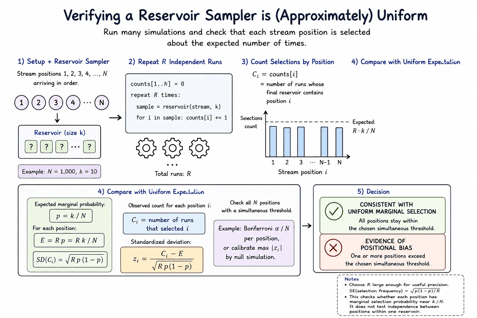
I would run the reservoir sampler many independent times on the same stream of N positions with reservoir size k. For every position i, I would count how many final reservoirs contain it. Under uniform marginal selection, each position has probability p = k / N, so its expected count over R runs is E = Rk / N. I would standardize each count using its binomial standard deviation and compare all positions with one simultaneous threshold. If every position stays inside that threshold, the results are consistent with uniform marginal selection. If one or more positions exceed it, I would investigate possible positional bias.

Detailed Explanation

See the Code while reading this explanation.

This question asks you to check whether a streaming sampler treats every input position fairly. Imagine the stream has N positions and the final reservoir keeps k items. Run the sampler many times with fresh random choices. For each position, count how many runs include it in the final reservoir. If the sampler is fair, every position should appear in about the same fraction of runs, namely k divided by N. The key is to allow normal random variation while still spotting positions that appear too often or too rarely.

Useful Questions to Ask the Interviewer
  1. Should I check only the marginal selection frequency of each stream position?
  2. Do you want a fixed significance level for the simultaneous comparison?
How would you verify that a reservoir sampler selects items close to uniformly? diagram
How to Explain It in an Interview

I would treat this as a probabilistic evaluation of the reservoir sampler. The system under test is the sampler itself. The input is a stream with positions 1 through N, and the reservoir has size k. The main property I want to check is whether every position has marginal selection probability close to k / N.

First, I create a count array with one entry for every stream position. I set every count to zero. Then I run the sampler R independent times. After each run, I look at the final reservoir. For every position included in that reservoir, I add one to its count.

For position i, let C_i be the number of runs that selected it. If the sampler is uniform, the expected marginal probability is p = k / N. The expected count is E = R p = Rk / N.

Across independent runs, the count for one fixed position follows a binomial model with standard deviation sqrt(R p times (1 minus p)). I can therefore compute a standardized deviation for each position as z_i = (C_i minus E) divided by sqrt(R p times (1 minus p)). This tells me how far the observed count is from the expected count in units of normal random variation.

Because I inspect all N positions, I should not judge every position with an unrelated single position threshold. That would increase the chance of a false alarm. I would use a simultaneous rule. A simple conservative choice is a Bonferroni threshold using alpha divided by N for each position. Another choice is to simulate correct uniform reservoir samples and calibrate the null distribution of the largest absolute z value.

The success result is not that the sampler is proven uniform. The result is that the observed counts are consistent with uniform marginal selection at the chosen threshold. If one or more positions exceed the simultaneous threshold, that is evidence of possible positional bias and I would investigate the sampler implementation.

The repeated runs should use independent random draws. For a repeatable automated test, I can seed the random number generator while still giving each run new random draws from that generator. The count array is reset before each complete evaluation. There is no external service or database in this test boundary, so no mock or integration dependency is needed.

The main tradeoff is R. A larger R gives more precise frequency estimates, but it also increases evaluation time. The standard error of the observed selection frequency for one position is sqrt(p times (1 minus p) divided by R).

An important limitation is that this test checks each position's marginal selection probability. Positions inside one reservoir are not independent because exactly k positions are selected. This evaluation does not test independence between positions within one reservoir. For small R or very small expected counts, I would prefer direct null simulation over relying only on a normal approximation.

Key Insight / Why This Solution Works
  1. Fix the stream length N, reservoir size k, number of independent runs R, and significance level alpha.
  2. Create counts for positions 1 through N and set every count to zero.
  3. Repeat R times. Run the reservoir sampler on the same N position stream. For every position in the final reservoir, increase its count by one.
  4. For each position i, record C_i = counts[i].
  5. Compute the expected marginal probability p = k / N.
  6. Compute the expected count E = R p = Rk / N.
  7. Compute the marginal count standard deviation sqrt(R p times (1 minus p)).
  8. Compute z_i = (C_i minus E) divided by sqrt(R p times (1 minus p)) for every position.
  9. Check all N positions with one simultaneous decision rule. A simple choice is a two sided Bonferroni threshold with alpha divided across N positions. Another choice is to calibrate the largest absolute z value with null simulation.
  10. If all positions remain inside the chosen simultaneous threshold, report that the results are consistent with uniform marginal selection. If any position exceeds the threshold, report evidence of possible positional bias.
Code
import math
import random
from statistics import NormalDist


def reservoir_sample(stream, k, rng):
    # Build the first reservoir from the first k stream positions.
    reservoir = list(stream[:k])

    # Give every later position the standard reservoir replacement chance.
    for index in range(k, len(stream)):
        replacement = rng.randint(0, index)
        if replacement < k:
            reservoir[replacement] = stream[index]

    return reservoir


def verify_uniform_selection(n=1000, k=10, runs=100000, alpha=0.05, seed=7):
    # Validate the test setup before running the simulation.
    if not 0 < k < n:
        raise ValueError("This statistical check requires 0 < k < n")
    if runs <= 0:
        raise ValueError("runs must be positive")
    if not 0 < alpha < 1:
        raise ValueError("alpha must be between 0 and 1")

    # Use one repeatable random generator while taking fresh draws on every run.
    rng = random.Random(seed)
    stream = list(range(n))
    counts = [0] * n

    # Run the sampler many times and count final reservoir membership by position.
    for _ in range(runs):
        sample = reservoir_sample(stream, k, rng)
        for position in sample:
            counts[position] += 1

    # Compute the expected marginal count and its binomial standard deviation.
    p = k / n
    expected = runs * p
    standard_deviation = math.sqrt(runs * p * (1 - p))

    # Standardize every position so deviations share one comparable scale.
    z_values = [(count - expected) / standard_deviation for count in counts]

    # Split the total error rate across all positions and both distribution tails.
    tail_probability = alpha / (2 * n)
    z_limit = NormalDist().inv_cdf(1 - tail_probability)
    max_abs_z = max(abs(value) for value in z_values)

    # This assertion checks consistency with uniform marginal selection.
    assert max_abs_z <= z_limit, (
        f"Possible positional bias: max absolute z = {max_abs_z:.3f}, limit = {z_limit:.3f}"
    )

    # Return useful diagnostics so a failure can be investigated.
    return {
        "expected_count": expected,
        "standard_deviation": standard_deviation,
        "max_abs_z": max_abs_z,
        "z_limit": z_limit,
    }


if __name__ == "__main__":
    result = verify_uniform_selection()
    print(result)
Why Interviewers Ask This

The interviewer wants to see whether I can test a random algorithm without expecting identical results on every run. They also want to see whether I can define the correct expected probability, measure normal random variation, and avoid claiming that a statistical check proves perfect uniformity.

Common interview mistakes

A common mistake is to expect every position to have exactly the same count. Random sampling naturally creates variation. Another mistake is to compare many positions with separate unadjusted thresholds, which raises the chance of false alarms. A third mistake is to use an ordinary Pearson chi square test with N minus 1 degrees of freedom on reservoir inclusion counts without accounting for dependence between positions within each run. It is also wrong to say that passing this check proves complete uniformity. The test checks marginal selection frequency, not independence between positions inside one reservoir. Finally, using too few runs can make the result too noisy to be useful.

Interview tip

Start with the simple idea: run the sampler many times and count how often each stream position appears. Then state the expected probability k / N and expected count Rk / N. Explain that random variation is normal, so you standardize the deviations and use one simultaneous threshold across all positions. End by saying that a pass means the results are consistent with uniform marginal selection, not that uniformity is mathematically proven.

Interviewer may ask next
What would you do if one stream position exceeds the simultaneous threshold?

I would treat that as evidence of possible positional bias, not immediate proof of a bug. The test boundary is still the reservoir sampler over repeated independent runs. I would first repeat the evaluation with enough R to reduce random noise and inspect whether the same position or region remains unusual. I would then review the sampler logic around replacement probabilities and index handling. The main tradeoff is that increasing R gives stronger evidence but costs more evaluation time.

How would you make this evaluation more reliable when N is large?

I would keep the same reservoir sampler boundary but use a simultaneous threshold that accounts for checking all N positions. Bonferroni is simple and conservative. A null simulation of the largest absolute standardized deviation can give a threshold that better matches the actual dependence structure. I would also choose R large enough for useful precision. The tradeoff is more computation because larger R and extra null simulations increase continuous integration time.

9. Remove duplicate strings from a stream.CodingEasyPerplexity

Question Details

Preserve the first occurrence of each string while processing the input incrementally rather than requiring the complete stream in memory.

Short Interview Answer (30-60 seconds)

I would process the stream one string at a time and keep a set called seen. The set stores the strings I have already emitted. For each incoming string, I check the set. If the string is new, I add it to seen and yield it immediately. If it is already present, I skip it. This preserves the first occurrence without storing the full stream. The expected time is O(n), and the extra space is O(u), where u is the number of unique strings.

Detailed Explanation

See the Code while reading this explanation.

The input is a stream of strings that arrive one at a time. We need to keep the first occurrence of each string and skip later copies. We should produce each useful result as soon as possible instead of waiting for the whole input. A set gives us a simple way to remember which strings were already emitted. This lets the solution work incrementally while keeping the original order of first occurrences. Memory grows with the number of unique strings, not with a stored copy of the whole stream.

Useful Questions to Ask the Interviewer
  1. Should string comparison be case-sensitive?
  2. Can the stream be very large or continue for an unknown amount of time?
  3. Should each unique string be produced immediately when its first occurrence arrives?
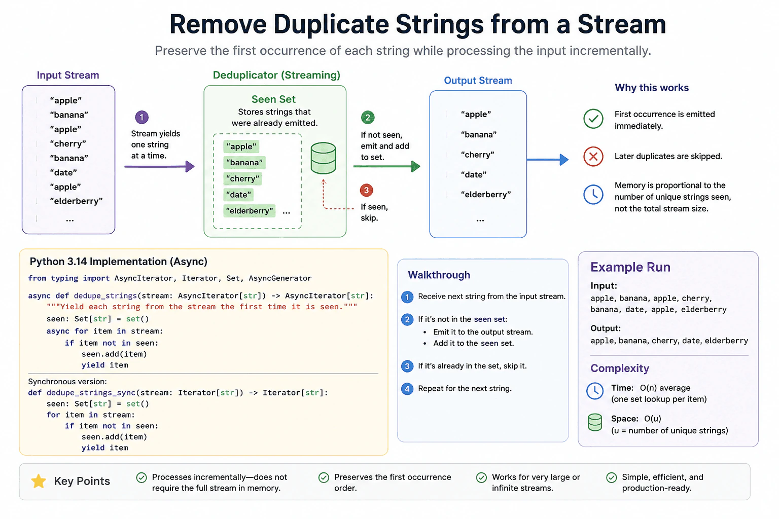
Remove duplicate strings from a stream. diagram
How to Explain It in an Interview
1. Understand the input and required output

The input provides one string at a time. The output must contain only the first occurrence of each string. The order of those first occurrences must stay the same. In the diagram, the input is apple, banana, apple, cherry, banana, date, apple, elderberry. The output is apple, banana, cherry, date, elderberry.

2. Use a set to remember emitted strings

Create a set named seen. A set stores unique values. Here, each value in seen means that string has already been emitted. The central invariant is: seen contains exactly the strings that have already passed to the output.

3. Process each string incrementally

Start with seen empty. Receive the next string. Check whether it is in seen. If it is not present, add it to the set and emit it. If it is already present, skip it. Then receive the next string. The algorithm never needs to collect the complete input stream first.

4. Walk through the example

Start with seen = {}. apple is new, so add it and emit apple. Now seen = {apple}. banana is new, so add it and emit banana. The next apple is already present, so skip it. cherry is new, so add and emit it. The next banana is skipped. date is new, so add and emit it. The next apple is skipped. elderberry is new, so add and emit it. The final output is apple, banana, cherry, date, elderberry.

5. Explain why it is correct

A string can be emitted only when it is missing from seen. As soon as the first occurrence is emitted, that string is added to seen. Every later copy therefore fails the new-string check and is skipped. Because values are processed in arrival order and emitted immediately, the first-occurrence order is preserved.

6. Explain the Python implementation

The diagram shows asynchronous and synchronous generator versions. The asynchronous version uses async for to receive values from an AsyncIterator[str]. The synchronous version uses a normal for loop over an Iterator[str]. Both keep the same seen set, perform the membership check, add new strings, and yield only first occurrences. The runnable example uses the synchronous version with the exact input from the diagram.

7. Explain complexity and the main limitation

Let n be the number of processed strings and u be the number of unique strings. Set membership and insertion are O(1) on average, so the expected total time is O(n). The seen set stores up to u strings, so auxiliary space is O(u). The stream itself does not need to be stored. A very large or infinite stream can be processed incrementally, but memory can continue growing if new unique strings continue arriving.

Key Insight / Why This Solution Works

The key idea is to remember only whether each string has already been emitted. The seen set provides that state. Its invariant is simple: after every processed item, seen contains exactly the unique strings emitted so far. When the next string arrives, the algorithm first checks membership. A new string is added and emitted. A string already in the set is skipped. This fits streaming input because each item can be handled immediately without waiting for the complete stream.

Code
from typing import AsyncIterator, Iterator, Set


async def dedupe_strings(stream: AsyncIterator[str]) -> AsyncIterator[str]:
    """Yield each string from the async stream the first time it is seen."""
    # Store exactly the strings that have already been emitted.
    seen: Set[str] = set()

    # Read one string at a time so the complete stream is never collected first.
    async for item in stream:
        # A string already in seen is a later duplicate, so do not emit it again.
        if item in seen:
            continue

        # Record the first occurrence before yielding it.
        # This keeps the seen-set invariant correct whenever iteration pauses.
        seen.add(item)

        # Emit the first occurrence immediately.
        yield item


def dedupe_strings_sync(stream: Iterator[str]) -> Iterator[str]:
    """Yield each string from the stream the first time it is seen."""
    # Store exactly the strings that have already been emitted.
    seen: Set[str] = set()

    # Process each incoming string incrementally.
    for item in stream:
        # Skip a value when its first occurrence was already emitted.
        if item in seen:
            continue

        # Remember this new value so later copies can be recognized.
        seen.add(item)

        # Emit the first occurrence without waiting for the rest of the input.
        yield item


def main() -> None:
    # Use the exact example shown in the diagram.
    input_stream: list[str] = [
        "apple",
        "banana",
        "apple",
        "cherry",
        "banana",
        "date",
        "apple",
        "elderberry",
    ]

    # Materialize only the small example output for display.
    # The deduplication generator itself still works incrementally.
    output: list[str] = list(dedupe_strings_sync(iter(input_stream)))

    # Expected output: ['apple', 'banana', 'cherry', 'date', 'elderberry']
    print(output)


if __name__ == "__main__":
    main()
Time & Space Complexity

Let n be the number of strings processed and u be the number of unique strings. Each input string needs one membership check. A new string also needs one insertion. Python set lookup and insertion are O(1) on average, so the expected total time is O(n). The seen set can contain u unique strings, so auxiliary space is O(u). The algorithm does not store the complete input stream, but its memory can keep growing when new unique strings keep arriving.

Where it is used

This pattern is useful in streaming pipelines where repeated string values should be ignored after their first appearance. Examples include filtering repeated event identifiers, repeated messages, or repeated record keys while data is arriving. It is especially useful when the complete input is too large to load before processing.

Why Interviewers Ask This

This question checks whether the candidate recognizes a streaming deduplication pattern and chooses a suitable data structure. It tests whether they can preserve first-occurrence order without collecting the complete stream. It also checks duplicate handling, generator behavior, and the ability to maintain a simple invariant. Finally, the interviewer can see whether the candidate explains hash-set complexity accurately as expected O(n) time with O(u) auxiliary space.

Common interview mistakes

One mistake is collecting the full stream before removing duplicates. That loses the incremental processing benefit. Another is converting the whole input directly to a set, which does not represent the required first-occurrence output flow and also consumes the input first. A candidate may also forget to add a new string to seen, causing later copies to be emitted again. Using a list for membership checks makes each lookup slower as the stored values grow. Another mistake is claiming guaranteed O(n) time instead of expected O(n) time for a hash-set solution. Finally, claiming O(1) extra space is wrong because seen grows with the number of unique strings.

Interview tip

Explain the invariant first: seen contains exactly the strings already emitted. Then trace one new string and one duplicate. This quickly shows why the first occurrence passes through and every later copy is skipped.

Interviewer may ask next
What happens if the stream is infinite and keeps producing new unique strings?

The algorithm can still process the stream incrementally, but the seen set keeps growing because exact deduplication must remember every previously emitted unique string. The basic algorithm remains the same. If in-memory space is limited, the membership state can be moved to an external store. That preserves exact duplicate checking but adds storage and I/O cost. The original in-memory version has expected O(n) processing time for n processed items and O(u) auxiliary memory for u unique strings.

Does this solution preserve the original order of the unique strings?

Yes. A new string is yielded at the moment its first occurrence arrives. The set is used only for membership checks. We never iterate over the set to build the output. Therefore the emitted sequence keeps the original first-occurrence order. The expected time remains O(n), and the auxiliary space remains O(u).

10. Implement reservoir sampling over an unknown-size or infinite stream in one pass using O(k) memory.CodingMediumPerplexity

Question Details

Select a sample of size k from a stream whose final length is not known in advance, process every item at most once, and keep auxiliary memory bounded by the sample size.

Short Interview Answer (30-60 seconds)

I would use reservoir sampling. I first store the first k items in a reservoir. For each later item at position i, I draw j uniformly from 1 through i. If j is at most k, I replace reservoir slot j. Otherwise, I discard the new item. After n >= k items, each seen item has probability k / n of being selected. The algorithm takes O(n) time for n processed items and O(k) auxiliary space.

Detailed Explanation

See the Code while reading this explanation.

The stream arrives one item at a time, and we do not know its final size. We need to keep exactly k sampled items without saving the whole stream. Reservoir sampling fits this problem because its memory stays limited to k items. We first fill the reservoir. After that, each new item gets a fair chance to replace one stored item. For a finite stream, returning exactly k items requires at least k input items. A truly infinite stream needs an external stopping point before this function can return.

Useful Questions to Ask the Interviewer
  1. Can I assume a finite stream contains at least k items?
  2. For a truly infinite stream, should I expose the current reservoir when an external stop or snapshot is requested?
Implement reservoir sampling over an unknown-size or infinite stream in one pass using O(k) memory. diagram
How to Explain It in an Interview
1. Understand the input and output

The input is a stream and an integer k. Items arrive one by one. The final number of items may be unknown. The output is a list containing k sampled items when a finite stream has at least k items. We only keep the reservoir, so memory does not grow with the length of the stream.

2. Fill the reservoir

Store the first k items directly. In the diagram example, k = 3. Item A gives [A, –, –]. Item B gives [A, B, –]. Item C gives [A, B, C]. At this point the reservoir is full.

3. Process every later item

Suppose the current item is at one-based position i. Draw j uniformly from 1 through i. If j <= k, replace reservoir position j with the new item. If j > k, discard the new item. This gives later items a decreasing chance to enter the sample while keeping the reservoir size fixed.

4. Walk through the exact example

For item D at i = 4, the illustrated random draw is j = 2. Because 2 <= 3, replace slot 2. The reservoir becomes [A, D, C]. For E at i = 5, j = 5. Because 5 > 3, discard E, so the reservoir stays [A, D, C]. For F at i = 6, j = 1. Because 1 <= 3, replace slot 1. The shown reservoir becomes [F, D, C]. These j values are one valid random outcome, not fixed results.

5. Explain why it is correct

After seeing n >= k items, every seen item has probability k / n of being in the reservoir. The first k items start inside the reservoir, but later replacement steps reduce their survival probability correctly. A later item enters with probability k / i when it arrives. The same rule keeps all seen items equally likely. Therefore, after any finite prefix of length n >= k, the reservoir is a uniform sample over all k-item subsets of those n items.

6. Explain the implementation and limits

The Python code counts items with one-based positions. It appends the first k items. For every later item, randbelow(i) produces a value from 0 through i - 1, so adding 1 gives j from 1 through i. A replacement uses reservoir[j - 1] because Python lists use zero-based indices. Negative k is invalid. k = 0 returns an empty sample. A finite stream shorter than k raises an error. For k > 0, a truly infinite iterator never reaches the final return unless processing is externally stopped.

7. Explain complexity

If n items are processed, the running time is O(n) because each item is handled once. The reservoir stores at most k items, so auxiliary space is O(k). The algorithm does not need to know n in advance.

Key Insight / Why This Solution Works

The key idea is to keep only k items while giving every item seen so far the same chance to be selected. The invariant is: after processing n >= k items, the reservoir is a uniform sample of size k from those n items. The first k items fill the reservoir. For item i > k, drawing j uniformly from 1 through i and replacing only when j <= k gives that new item probability k / i of entering. The replacement rule also reduces the survival probability of older items by the exact amount needed to keep all items equally likely.

Code
from __future__ import annotations

from collections.abc import Callable, Iterable
from secrets import randbelow
from typing import TypeVar

T = TypeVar("T")


def reservoir_sample(
    stream: Iterable[T],
    k: int,
    random_below: Callable[[int], int] = randbelow,
) -> list[T]:
    """Return a uniform random sample of size k from a finite stream."""
    # A negative sample size is invalid.
    if k < 0:
        raise ValueError("k must be non-negative")

    # A sample of size zero is valid and needs no stream processing.
    if k == 0:
        return []

    # The reservoir is the only storage that grows with k.
    reservoir: list[T] = []

    # Start counting at one because the reservoir formula uses positions 1..i.
    for i, item in enumerate(stream, start=1):
        # The first k items fill the reservoir directly.
        if i <= k:
            reservoir.append(item)
            continue

        # random_below(i) returns 0..i-1, so adding one gives j in 1..i.
        j = random_below(i) + 1

        # Only positions 1..k map to reservoir slots. Larger j values discard item.
        if j <= k:
            # Python lists are zero-based, so reservoir position j is index j - 1.
            reservoir[j - 1] = item

    # Returning exactly k items requires at least k items in the finite input.
    if len(reservoir) < k:
        raise ValueError("stream contains fewer than k items")

    # After n >= k processed items, this is a uniform k-sample of those n items.
    return reservoir


def main() -> None:
    # This is the exact stream used by the diagram walkthrough.
    stream = ["A", "B", "C", "D", "E", "F"]
    k = 3

    # The diagram uses j values 2, 5, and 1 for i = 4, 5, and 6.
    # random_below must return j - 1, so these values are 1, 4, and 0.
    illustrated_draws = iter([1, 4, 0])

    def deterministic_random_below(upper_bound: int) -> int:
        # This deterministic fake reproduces only the diagram's illustrated trace.
        value = next(illustrated_draws)

        # Keep the fake under the same 0..upper_bound-1 contract as randbelow.
        if not 0 <= value < upper_bound:
            raise ValueError("deterministic random value is outside the valid range")
        return value

    # Run the same reservoir algorithm with deterministic draws for this example.
    sample = reservoir_sample(stream, k, deterministic_random_below)
    print(sample)  # ['F', 'D', 'C']


if __name__ == "__main__":
    main()
Time & Space Complexity

Let n be the number of items processed. Time is O(n) because the algorithm handles each item once and does constant work per processed item in the illustrated model. Auxiliary space is O(k) because the reservoir contains at most k references. It does not store the full stream. For a truly infinite stream, n keeps growing and the exhaustion-based function does not naturally finish. After any finite prefix with n >= k, the current reservoir is still a valid uniform k-sample.

Where it is used

Reservoir sampling is useful when data arrives as a stream and storing everything is too expensive. Examples include sampling records from a very large log, taking a random sample from events arriving over time, or keeping a small representative sample while reading data whose final length is not known.

Why Interviewers Ask This

This problem tests whether you can design an algorithm when the input size is unknown and memory is limited. The interviewer wants to see whether you recognize reservoir sampling, maintain a clear probability invariant, and translate one-based probability reasoning into correct zero-based Python indexing. It also tests whether you can explain O(n) processing and O(k) auxiliary space accurately, handle k edge cases, and notice the important termination difference between an unknown finite stream and a truly infinite stream.

Common interview mistakes

A common mistake is choosing a random reservoir slot for every new item. That makes later items too likely to survive. Another mistake is drawing only from 1 through k instead of 1 through the current position i. Candidates also sometimes forget that j is one-based while a Python list index is zero-based. Another mistake is storing the whole stream, which breaks the O(k) memory goal. It is also incorrect to return fewer than k items silently when a finite stream is shorter than k, or to say an exhaustion-based function returns from a truly infinite iterator without an external stopping condition.

Interview tip

Explain the invariant before writing code: after n >= k items, every seen item must have probability k / n of being in the reservoir. Then show how drawing j from 1..i and replacing only when j <= k preserves that invariant.

Interviewer may ask next
How would you use this with a truly infinite stream?

The reservoir update rule does not change. After every finite prefix containing at least k items, the current reservoir is a valid uniform k-sample of the items seen so far. The important change is the output behavior. An exhaustion-based function cannot naturally return because the stream never ends. I would expose a snapshot when an external stop, cancellation, time limit, or other application-defined boundary occurs. Processing m items takes O(m) time, and the reservoir uses O(k) auxiliary space.

Why do we draw j from 1 through i instead of directly replacing a random reservoir slot?

The range 1..i controls whether the new item enters at all. It enters only when j <= k, so its probability of entering is k / i. If it enters, each of the k slots is equally likely to be replaced. This keeps old and new items balanced so every item seen so far has the same probability of remaining. Drawing only a reservoir slot would force every new item into the sample and would destroy uniform sampling. Time remains O(n) and auxiliary space remains O(k).

More questions load as you scroll

Disclaimer: This interview guide is for educational and informational purposes only. It is designed to help readers prepare, but it does not guarantee any interview result, hiring decision, offer, or outcome. Interview questions, hiring criteria, and preferred answers can vary by employer, interviewer, industry, location, and time. The examples and explanations reflect the authors' research and judgment, are provided without warranties of any kind, and should not be treated as the only correct approach. Diagrams are simplified illustrations intended to highlight the main components and their interactions; actual systems and implementations may be more complex. Alternative approaches may be equally valid or better suited to a particular question, context, or interviewer. To the fullest extent permitted by applicable law, the author, contributors, and publisher are not liable for decisions made, actions taken, or losses incurred based on this guide.

Company Notice: This guide is an independent educational resource and is not affiliated with, endorsed by, sponsored by, or approved by the company named in this guide. Company names are used only to identify interview experiences commonly reported by candidates. Interview practices can change without notice, and inclusion of company-specific content does not mean these questions are official, complete, or guaranteed to be asked. To the fullest extent permitted by law, the author, contributors, and publisher are not responsible for outcomes related to use of this material.