Apple Python Developer Interview Questions & Answers

apple icon

Questions with Detailed ExplanationsWith Detailed Explanations

(Last Updated: August 28, 2026)

11. How would you implement wildcard and null-aware lookup logic in Python?Language SpecificHardApple

Question Details

Explain Python representation choices for records whose lookup dimensions may be exact values, wildcards, or nulls. Cover matching order, trie-like indexing, ambiguity, missing fields, and performance tradeoffs.

Short Interview Answer (30-60 seconds)

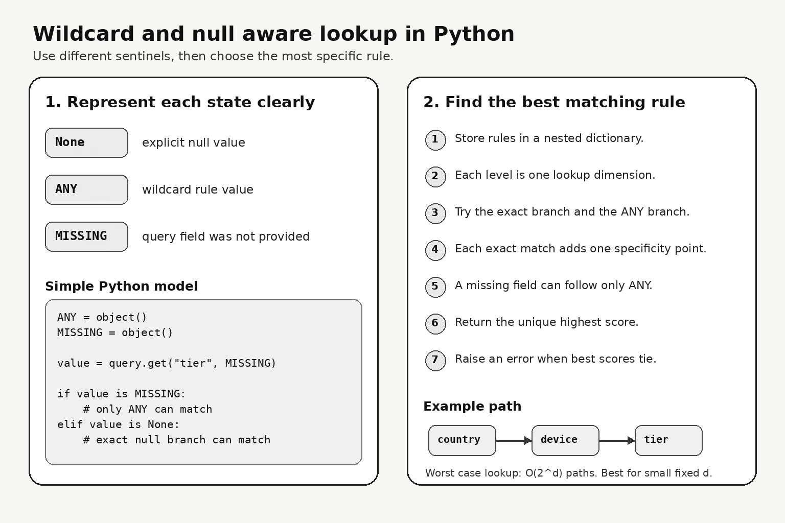
I would use None only for an explicit null value and use private sentinel objects for a wildcard and a missing query field. I would store rules in a nested dictionary with one level per lookup dimension. During lookup, I would explore the exact branch and the wildcard branch, count exact matches, and return the unique rule with the highest specificity. A missing query field can match only a wildcard. If several different rules have the same best specificity, I would raise an ambiguity error.

Detailed Explanation

See the Code while reading this explanation.

I would represent exact values, nulls, wildcards, and missing fields as separate states. None means an explicit null. A private ANY sentinel means any value. A separate MISSING sentinel means the query did not provide that field. This matters because query.get alone cannot distinguish a missing key from a key whose value is None.

Useful Questions to Ask the Interviewer
  1. Should I focus on Python language behavior, or also explain the runtime and standard library?
  2. Which Python version and execution environment should I assume?
  3. Would you like a small code example together with production tradeoffs and edge cases?

I would index rules in a nested dictionary with one level for each lookup dimension. A rule that omits a dimension uses ANY for that level. During lookup, an exact branch, including a None branch, adds one specificity point. An ANY branch adds no point. A missing query field can follow only ANY because there is no exact value to compare.

The lookup returns the unique rule with the highest specificity. If different rules share the best score, it raises an ambiguity error instead of depending on insertion order. Building the index costs O(n times d) time and up to O(n times d) memory, where n is the number of rules and d is the number of dimensions. Prefix sharing can reduce memory. Lookup may explore up to O(2 to the power d) paths in the worst case, so this design works best with a small, fixed number of dimensions.
How would you implement wildcard and null-aware lookup logic in Python? diagram
Example

The code uses ANY as the wildcard sentinel, MISSING as the absent query field sentinel, and LEAF as a private storage key for rules. None remains an ordinary exact lookup value. Rules are inserted into a nested dictionary in a fixed dimension order. An omitted rule dimension becomes ANY. Lookup explores an exact branch when the query contains the field and also explores an ANY branch when one exists. Each exact branch adds one specificity point. Missing query fields can follow only ANY. The code returns the unique rule with the highest score and raises AmbiguousMatchError when different rules share that score. Index construction uses O(n times d) time and up to O(n times d) memory. Worst case lookup explores O(2 to the power d) paths.

Code
from dataclasses import dataclass
from typing import Any as TypingAny


# Private sentinel for a wildcard rule value.
ANY = object()

# Private sentinel for a query field that is not present.
MISSING = object()

# Private sentinel used to store rules at a leaf node.
LEAF = object()


class AmbiguousMatchError(Exception):
    """Raised when different rules have the same best specificity."""


@dataclass(frozen=True)
class Rule:
    name: str
    values: dict[str, TypingAny]
    result: str


class RuleIndex:
    def __init__(self, dimensions: tuple[str, ...]) -> None:
        # The dimension order must be stable for insertion and lookup.
        self.dimensions = dimensions
        self.root: dict[TypingAny, TypingAny] = {}

    def add(self, rule: Rule) -> None:
        """Insert one rule into the nested dictionary index."""
        node = self.root

        for dimension in self.dimensions:
            # An omitted rule dimension means wildcard behavior.
            key = rule.values.get(dimension, ANY)
            node = node.setdefault(key, {})

        # More than one rule may occupy the same leaf.
        node.setdefault(LEAF, []).append(rule)

    def lookup(self, query: dict[str, TypingAny]) -> Rule | None:
        """Return the unique most specific rule for the query."""
        matches: list[tuple[int, Rule]] = []

        def visit(
            node: dict[TypingAny, TypingAny],
            depth: int,
            specificity: int,
        ) -> None:
            # All dimensions have been processed.
            if depth == len(self.dimensions):
                for rule in node.get(LEAF, []):
                    matches.append((specificity, rule))
                return

            dimension = self.dimensions[depth]
            query_value = query.get(dimension, MISSING)

            # A present query field may follow its exact branch.
            # None is treated as an exact value here.
            if query_value is not MISSING and query_value in node:
                visit(
                    node[query_value],
                    depth + 1,
                    specificity + 1,
                )

            # A wildcard can match any value and can also match a missing field.
            if ANY in node:
                visit(
                    node[ANY],
                    depth + 1,
                    specificity,
                )

        visit(self.root, 0, 0)

        if not matches:
            return None

        best_score = max(score for score, _ in matches)
        best_rules = [rule for score, rule in matches if score == best_score]

        # Remove repeated references to the same Rule object only.
        unique_rules: list[Rule] = []
        seen_ids: set[int] = set()

        for rule in best_rules:
            rule_id = id(rule)
            if rule_id not in seen_ids:
                seen_ids.add(rule_id)
                unique_rules.append(rule)

        if len(unique_rules) > 1:
            names = ", ".join(sorted(rule.name for rule in unique_rules))
            raise AmbiguousMatchError(f"Ambiguous rules at specificity {best_score}: {names}")

        return unique_rules[0]


if __name__ == "__main__":
    index = RuleIndex(("country", "device", "tier"))

    index.add(
        Rule(
            name="us mobile null tier",
            values={
                "country": "US",
                "device": "mobile",
                "tier": None,
            },
            result="rule A",
        )
    )

    index.add(
        Rule(
            name="us wildcard device and tier",
            values={"country": "US"},
            result="rule B",
        )
    )

    index.add(
        Rule(
            name="global default",
            values={},
            result="rule C",
        )
    )

    first = index.lookup({"country": "US", "device": "mobile", "tier": None})
    second = index.lookup({"country": "US", "device": "desktop"})
    third = index.lookup({"country": "CA"})

    print(first.result if first else None)
    print(second.result if second else None)
    print(third.result if third else None)
Where it is used

This design is useful for configuration selection, feature rules, pricing rules, routing policies, access rules, and content selection. For example, one rule can match country US, device mobile, and an explicit null customer tier. Another rule can match country US with any device and any tier. A final wildcard rule can act as the global default.

Why Interviewers Ask This

Interviewers ask this question to test whether a candidate can represent exact values, explicit null values, wildcards, and missing fields without confusing them. It also evaluates Python data structure knowledge, deterministic matching rules, ambiguity handling, and judgment about lookup speed and memory use.

Common interview mistakes

Common mistakes include using None for both null and wildcard, using query.get without a missing sentinel, treating a missing field as an explicit null, returning the first match found, and using insertion order to hide ambiguous rules. Another mistake is claiming lookup always costs O(d). Exact and wildcard branches may both exist at each level, so worst case lookup can explore O(2 to the power d) paths. It is also a mistake to ignore the memory used by nested dictionary nodes.

Interview tip

Start with the representation rule. Say that None means explicit null, ANY means wildcard, and MISSING means an absent query field. Then explain specificity scoring, ambiguity handling, and the worst case branching and memory costs.
Interviewer may ask next
What happens when a query field is missing but a rule stores None for that dimension?

The None branch does not match. A missing field is represented by MISSING, while None is an explicit exact value. The lookup can follow an ANY branch when one exists. This distinction matters because treating absence as null could select a rule that the caller did not request.

When would you use a linear scan instead of the nested dictionary index?

I would use a linear scan when the rule set is small, rules change often, or the number of dimensions makes index memory and wildcard branching too expensive. A scan costs O(n times d) for each lookup but is simpler to update and inspect. The nested dictionary index is more useful when lookups are frequent, dimensions are few and stable, and shared prefixes reduce repeated work.

12. How would you structure Python parsing code for an event stream that later needs random-access reads?Language SpecificHardApple

Question Details

Explain Python parsing boundaries, schema handling, incremental processing, indexing metadata, error isolation, validation, memory use, and how implementation choices change when random-access reads are later required.

Short Interview Answer (30-60 seconds)

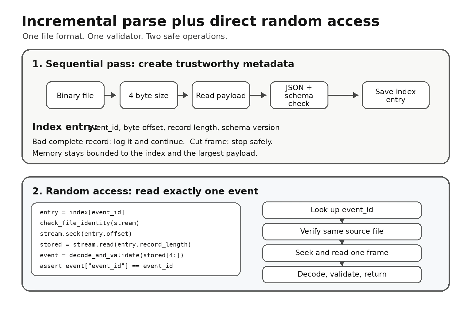
I would parse the stream incrementally and build a compact index during the same pass. Each valid event would store its identifier, byte offset, record length, and schema version. Later, Python can open the immutable source in binary mode, seek to that offset, read one framed record, and run the same decoder and validator. I would rebuild the index whenever the source changes because saved offsets are valid only for the exact bytes that were indexed.

Detailed Explanation

See the Code while reading this explanation.

I would separate sequential parsing from random access. The sequential layer reads one framed record at a time and yields validated events, so Python keeps only the current payload in memory. Each record has a fixed four byte header that stores the payload length. This stable boundary tells the parser where one event ends and the next begins.

Useful Questions to Ask the Interviewer
  1. Should I focus on Python language behavior, or also explain the runtime and standard library?
  2. Which Python version and execution environment should I assume?
  3. Would you like a small code example together with production tradeoffs and edge cases?

For every valid event, I would store compact metadata: the event identifier, byte offset, total record length, and schema version. Invalid JSON, unsupported schemas, missing fields, and duplicate identifiers can be isolated at a complete record boundary. A truncated header or payload is different because the next boundary is unknown, so the scan must stop safely.

A later lookup opens the immutable source in binary mode, seeks to the saved byte offset, reads exactly one frame, and runs the same decoder and validator. Building the index takes one sequential pass. Each lookup reads one record, while memory use is the index plus the largest payload being processed. Production code should treat indexed files as immutable, store source identity metadata, and rebuild the index after replacement, truncation, or rewriting.

How would you structure Python parsing code for an event stream that later needs random-access reads? diagram
Example

The code writes every JSON event as a four byte length header followed by one payload. The index builder opens the file in binary mode and scans it once. It validates each complete record and stores compact metadata only for valid unique event identifiers. Invalid payloads are reported while later framed records continue. Truncated framing or an unreasonable payload length stops the scan because continuing would not be safe. The code records file identity metadata from the open file before and after indexing. A lookup opens the source, verifies the identity on that same file handle, seeks to the saved byte offset, reads the exact frame, checks the stored length, and applies the same decoder and validator used during indexing.

Code
import json
import os
import struct
import tempfile
from dataclasses import dataclass
from pathlib import Path
from typing import Any, BinaryIO


# Each record begins with an unsigned four byte payload length.
HEADER = struct.Struct(">I")

# Reject unreasonable payload sizes before allocating large byte objects.
MAX_PAYLOAD_BYTES = 1_000_000


@dataclass(frozen=True)
class FileIdentity:
    # These values detect common replacement, truncation, and rewrite cases.
    device: int
    inode: int
    size: int
    modified_ns: int


@dataclass(frozen=True)
class IndexEntry:
    # Byte position where the record header starts.
    offset: int
    # Total bytes occupied by the header and payload.
    record_length: int
    # Schema version used to validate the event.
    schema_version: int


@dataclass(frozen=True)
class EventIndex:
    # Lookup metadata for valid events.
    entries: dict[str, IndexEntry]
    # Identity of the exact source file used to build the index.
    source_identity: FileIdentity


def identity_from_stream(stream: BinaryIO) -> FileIdentity:
    # Use the open file descriptor to avoid checking a different path target.
    stat = os.fstat(stream.fileno())
    return FileIdentity(
        device=stat.st_dev,
        inode=stat.st_ino,
        size=stat.st_size,
        modified_ns=stat.st_mtime_ns,
    )


def validate_event(event: dict[str, Any]) -> None:
    # This example supports one explicit schema version.
    if event.get("schema_version") != 1:
        raise ValueError("unsupported schema version")

    event_id = event.get("event_id")
    if not isinstance(event_id, str) or not event_id:
        raise ValueError("event_id must be a nonempty string")

    event_type = event.get("type")
    if not isinstance(event_type, str) or not event_type:
        raise ValueError("type must be a nonempty string")

    # bool is a subclass of int, so reject it explicitly.
    value = event.get("value")
    if isinstance(value, bool) or not isinstance(value, int):
        raise ValueError("value must be an integer")


def decode_and_validate(payload: bytes) -> dict[str, Any]:
    # Both indexing and random access use this exact parsing boundary.
    decoded = json.loads(payload.decode("utf8"))

    if not isinstance(decoded, dict):
        raise ValueError("event must be a JSON object")

    validate_event(decoded)
    return decoded


def write_event_stream(path: Path, events: list[dict[str, Any]]) -> None:
    # Write stable framed records so byte offsets remain meaningful.
    with path.open("wb") as stream:
        for event in events:
            payload = json.dumps(
                event,
                separators=(",", ":"),
            ).encode("utf8")

            if len(payload) > MAX_PAYLOAD_BYTES:
                raise ValueError("payload exceeds the configured limit")

            stream.write(HEADER.pack(len(payload)))
            stream.write(payload)


def build_index(path: Path) -> tuple[EventIndex, list[str]]:
    entries: dict[str, IndexEntry] = {}
    errors: list[str] = []

    with path.open("rb") as stream:
        identity_before = identity_from_stream(stream)

        while True:
            offset = stream.tell()
            header = stream.read(HEADER.size)

            if header == b"":
                break

            if len(header) != HEADER.size:
                errors.append(f"offset {offset}: truncated header")
                break

            payload_length = HEADER.unpack(header)[0]

            if payload_length > MAX_PAYLOAD_BYTES:
                errors.append(f"offset {offset}: payload length exceeds limit")
                break

            payload = stream.read(payload_length)

            if len(payload) != payload_length:
                errors.append(f"offset {offset}: truncated payload")
                break

            record_length = HEADER.size + payload_length

            try:
                event = decode_and_validate(payload)
                event_id = event["event_id"]

                if event_id in entries:
                    raise ValueError(f"duplicate event_id {event_id}")

                entries[event_id] = IndexEntry(
                    offset=offset,
                    record_length=record_length,
                    schema_version=event["schema_version"],
                )
            except (
                UnicodeDecodeError,
                json.JSONDecodeError,
                ValueError,
            ) as exc:
                # A complete bad record does not block later framed records.
                errors.append(f"offset {offset}: {exc}")

        identity_after = identity_from_stream(stream)

    if identity_after != identity_before:
        raise RuntimeError("source file changed while the index was built")

    return EventIndex(entries, identity_after), errors


def read_event(
    path: Path,
    event_index: EventIndex,
    event_id: str,
) -> dict[str, Any]:
    try:
        entry = event_index.entries[event_id]
    except KeyError as exc:
        raise KeyError(f"unknown event_id {event_id}") from exc

    with path.open("rb") as stream:
        # Verify the exact opened file before using saved offsets.
        if identity_from_stream(stream) != event_index.source_identity:
            raise RuntimeError("source file changed after indexing")

        stream.seek(entry.offset)
        stored = stream.read(entry.record_length)

        # Check the file again in case it changed during the read.
        if identity_from_stream(stream) != event_index.source_identity:
            raise RuntimeError("source file changed during random access")

    if len(stored) != entry.record_length:
        raise ValueError("indexed record is missing or truncated")

    if len(stored) < HEADER.size:
        raise ValueError("indexed record has no complete header")

    payload_length = HEADER.unpack(stored[: HEADER.size])[0]

    if payload_length > MAX_PAYLOAD_BYTES:
        raise ValueError("indexed payload length exceeds limit")

    payload = stored[HEADER.size :]

    if payload_length != len(payload):
        raise ValueError("indexed record length does not match its header")

    event = decode_and_validate(payload)

    if event["schema_version"] != entry.schema_version:
        raise ValueError("indexed schema version does not match the record")

    if event["event_id"] != event_id:
        raise ValueError("indexed event identifier does not match the record")

    return event


def main() -> None:
    events = [
        {
            "schema_version": 1,
            "event_id": "evt1",
            "type": "click",
            "value": 10,
        },
        {
            "schema_version": 1,
            "event_id": "evt2",
            "type": "purchase",
            "value": 25,
        },
        {
            "schema_version": 1,
            "event_id": "evt3",
            "type": "logout",
            "value": 0,
        },
    ]

    # A temporary directory makes the example runnable without setup.
    with tempfile.TemporaryDirectory() as directory:
        path = Path(directory) / "events.bin"
        write_event_stream(path, events)

        event_index, errors = build_index(path)

        print("Indexed event identifiers:", sorted(event_index.entries))
        print("Parsing errors:", errors)
        print(
            "Random access result:",
            read_event(path, event_index, "evt2"),
        )


if __name__ == "__main__":
    main()
Where it is used

This structure is useful for append only audit logs, telemetry archives, message capture files, local event stores, media metadata streams, and large import files. It fits systems that normally process events in order but later need direct reads for debugging, replay, support tools, or a user interface.

Why Interviewers Ask This

Interviewers ask this to test whether the candidate can separate parsing, validation, indexing, and lookup concerns in Python. It also checks understanding of generators, binary file offsets, schema versions, exception boundaries, bounded memory use, file mutation, and the tradeoff between sequential processing and later direct reads.

Common interview mistakes

Common mistakes include loading the full stream into a list, storing complete event objects instead of compact index metadata, recording text positions instead of byte offsets, opening the source in text mode, and trusting an unbounded length field. Another mistake is catching every exception around the whole file, which allows one bad record to stop all processing. Candidates may also continue after truncated framing even though the next boundary is unknown, validate only during the first pass, or reuse offsets after the source file has changed.

Interview tip

Start with the practical split: incremental parsing for normal processing and a byte offset index for later direct reads. Then explain stable framing, shared validation, record level error isolation, bounded memory use, and stale index detection.

Interviewer may ask next
What should the parser do if the final record is truncated?

It should stop at the incomplete frame and report its exact byte offset. A complete invalid payload can be isolated because the next record boundary is still known. A truncated header or payload does not provide a trustworthy next boundary. Continuing could interpret payload bytes as a new header. For a closed file, I would treat the tail as corrupt. For a file that is still receiving data, I would retain the incomplete tail and retry after more bytes arrive.

When should the index move from memory to persistent storage?

It should move to persistent storage when the index is too large for process memory, must survive restarts, or must be shared by several workers. Each stored entry still needs the event identifier, byte offset, record length, schema version, and source file identity. Persistent storage improves durability and shared access, but it adds storage operations and consistency work. An in memory dictionary is simpler for one process, while a database or embedded key value store is more suitable for a large or shared index.

13. How would you write Python for production ML tensor-shape code without hiding correctness errors?Language SpecificHardApple

Question Details

Explain Python practices for implementing ML tensor-shape logic, including explicit shape checks, readable variable names, validation, numerical edge cases, deterministic tests, and failure behavior when dimensions do not match.

Short Interview Answer (30-60 seconds)

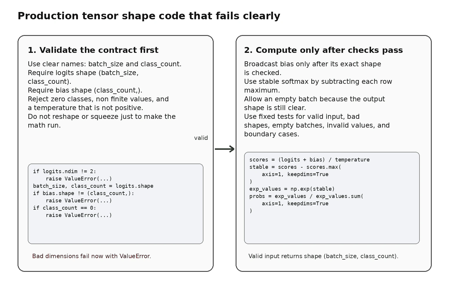
I would define the accepted shapes as part of the function contract and reject every unexpected shape before doing the calculation. I would use clear names such as batch_size and class_count, raise ValueError with the expected and received shapes, and allow broadcasting only after validating that it is intentional. I would also check important numerical conditions and use deterministic tests for valid input, mismatched dimensions, empty batches, invalid values, and boundary cases.

Detailed Explanation

See the Code while reading this explanation.

I would treat each tensor shape as part of the Python function contract. For example, logits must have shape batch_size by class_count, while bias must have shape class_count. I would validate rank and dimension sizes before NumPy performs arithmetic. I would not call reshape, flatten, or squeeze merely to make an operation succeed, because that can hide an upstream error.

Useful Questions to Ask the Interviewer
  1. Should I focus on Python language behavior, or also explain the runtime and standard library?
  2. Which Python version and execution environment should I assume?
  3. Would you like a small code example together with production tradeoffs and edge cases?

NumPy broadcasting can copy the logical effect of a smaller array across a larger one without physically copying every value. That behavior is useful here, but only after checking that bias has exactly one value per class.

The function should raise ValueError with the parameter name, expected shape, and received shape. It should also reject non real data, non finite values, an empty class dimension, and an invalid temperature. An empty batch can be allowed because its output shape remains well defined.

Deterministic tests should use fixed arrays and expected results. Shape checks take constant time because shape metadata is already stored. Value checks and softmax each scan all elements. The implementation therefore takes linear time and linear temporary memory. Converting input to float64 may also allocate a copy when the original type differs.

How would you write Python for production ML tensor-shape code without hiding correctness errors? diagram
Example

The function accepts logits with shape batch_size by class_count, bias with shape class_count, and one finite positive temperature value. It first rejects unsupported data types and converts valid real numeric inputs to float64. It then checks rank, requires at least one class, and verifies the exact bias shape before using intentional NumPy broadcasting. An empty batch is accepted and returns an empty float64 array with the same two dimensional shape. For a nonempty batch, the function rejects non finite inputs and catches overflow or invalid arithmetic while adding bias and dividing by temperature. It computes stable softmax by subtracting each row maximum before exponentiation. The deterministic tests verify output shape, row sums, equal score behavior, empty batch behavior, shape failures, non finite data, and invalid temperature. For N tensor elements, runtime is O(N). Temporary arrays and a required float64 conversion can use O(N) extra memory.

Code
import numpy as np


def _as_real_numeric_array(value: object, name: str) -> np.ndarray:
    """Convert supported real numeric input to a float64 NumPy array."""

    array = np.asarray(value)

    # Reject values that would hide data loss or unclear numeric behavior.
    if not np.issubdtype(array.dtype, np.number):
        raise TypeError(f"{name} must contain real numeric values")

    if np.issubdtype(array.dtype, np.complexfloating):
        raise TypeError(f"{name} must contain real numeric values")

    # This may return a view or allocate a new float64 array.
    return array.astype(np.float64, copy=False)


def validated_softmax(
    logits: np.ndarray,
    bias: np.ndarray,
    temperature: float = 1.0,
) -> np.ndarray:
    """Return softmax probabilities after explicit validation."""

    logits_array = _as_real_numeric_array(logits, "logits")
    bias_array = _as_real_numeric_array(bias, "bias")

    # Logits must have one row per batch item and one column per class.
    if logits_array.ndim != 2:
        raise ValueError(
            f"logits must have shape (batch_size, class_count), but received {logits_array.shape}"
        )

    # Bias must provide exactly one value for each class.
    if bias_array.ndim != 1:
        raise ValueError(f"bias must have shape (class_count,), but received {bias_array.shape}")

    batch_size, class_count = logits_array.shape

    # Softmax cannot produce class probabilities when no class exists.
    if class_count == 0:
        raise ValueError("logits must contain at least one class")

    # Check the exact permitted broadcasting shape.
    if bias_array.shape != (class_count,):
        raise ValueError(f"bias must have shape ({class_count},), but received {bias_array.shape}")

    # Temperature must be one scalar value rather than an array.
    temperature_array = np.asarray(temperature)
    if temperature_array.ndim != 0:
        raise ValueError("temperature must be one scalar value")

    try:
        temperature_value = float(temperature_array)
    except (TypeError, ValueError, OverflowError) as error:
        raise ValueError("temperature must be a real scalar value") from error

    if not np.isfinite(temperature_value) or temperature_value <= 0.0:
        raise ValueError(
            f"temperature must be finite and greater than zero, but received {temperature_value}"
        )

    # Reject invalid numbers before they spread through the result.
    if not np.isfinite(logits_array).all():
        raise ValueError("logits must contain only finite values")

    if not np.isfinite(bias_array).all():
        raise ValueError("bias must contain only finite values")

    # An empty batch has a valid and predictable output shape.
    if batch_size == 0:
        return np.empty((0, class_count), dtype=np.float64)

    # Catch overflow or invalid arithmetic instead of returning bad values.
    try:
        with np.errstate(over="raise", divide="raise", invalid="raise"):
            # Bias broadcasting is intentional and was validated above.
            scaled_scores = (logits_array + bias_array) / temperature_value

            # Subtract each row maximum before exponentiation for stability.
            stable_scores = scaled_scores - np.max(
                scaled_scores,
                axis=1,
                keepdims=True,
            )

            exponentials = np.exp(stable_scores)
            probabilities = exponentials / np.sum(
                exponentials,
                axis=1,
                keepdims=True,
            )
    except FloatingPointError as error:
        raise ValueError("logits, bias, and temperature produced invalid numeric values") from error

    # This assertion checks an internal invariant after caller validation.
    assert probabilities.shape == (batch_size, class_count)

    if not np.isfinite(probabilities).all():
        raise ValueError("softmax produced non finite probabilities")

    return probabilities


def run_deterministic_tests() -> None:
    """Run fixed tests that cover normal behavior and important failures."""

    logits = np.array(
        [
            [1.0, 2.0, 3.0],
            [2.0, 2.0, 1.0],
        ]
    )
    bias = np.array([0.1, 0.0, -0.1])

    probabilities = validated_softmax(logits, bias)

    assert probabilities.shape == (2, 3)
    np.testing.assert_allclose(
        probabilities.sum(axis=1),
        np.ones(2),
        rtol=1e-12,
        atol=1e-12,
    )

    equal_probabilities = validated_softmax(
        np.array([[5.0, 5.0, 5.0]]),
        np.zeros(3),
    )
    np.testing.assert_allclose(
        equal_probabilities,
        np.array([[1.0 / 3.0, 1.0 / 3.0, 1.0 / 3.0]]),
        rtol=1e-12,
        atol=1e-12,
    )

    empty_result = validated_softmax(
        np.empty((0, 3)),
        np.zeros(3),
    )
    assert empty_result.shape == (0, 3)

    failure_cases = [
        lambda: validated_softmax(np.ones(3), np.ones(3)),
        lambda: validated_softmax(np.ones((2, 3)), np.ones(2)),
        lambda: validated_softmax(np.ones((2, 0)), np.ones(0)),
        lambda: validated_softmax(
            np.array([[1.0, np.nan, 3.0]]),
            np.zeros(3),
        ),
        lambda: validated_softmax(np.ones((2, 3)), np.ones(3), 0.0),
    ]

    for failure_case in failure_cases:
        try:
            failure_case()
        except (TypeError, ValueError):
            pass
        else:
            raise AssertionError("Expected validation failure did not occur")


if __name__ == "__main__":
    run_deterministic_tests()
    print("All deterministic tests passed")
Where it is used

This pattern is used in model inference services, training loops, feature preprocessing, custom loss functions, attention code, batching logic, and model input adapters. It is most important at boundaries where tensors arrive from clients, data loaders, saved files, or separate pipeline stages.

Why Interviewers Ask This

Interviewers ask this to test whether a candidate treats tensor shapes as correctness rules instead of relying on accidental broadcasting or unclear reshape logic. They also evaluate exception design, NumPy runtime knowledge, numerical safety, deterministic testing, and judgment about validation cost in production.

Common interview mistakes

Common mistakes include reshaping or squeezing data until an operation runs, trusting every shape that NumPy can broadcast, comparing only the total number of elements, and returning a vague error. Other mistakes include silently converting complex values to real values, ignoring empty dimensions, accepting a non scalar temperature, and checking only successful examples. Using assert for caller supplied input is also wrong because Python can remove assertions when optimization is enabled.

Interview tip

State the exact tensor contract first. Then explain which broadcasting is intentional, which failures raise exceptions, how empty batches behave, and which deterministic tests protect the contract. Finish by separating constant time shape checks from linear value scans and temporary array allocations.

Interviewer may ask next
Why should caller supplied shape checks use ValueError instead of assert?

Use ValueError because caller supplied validation must run in every normal Python execution mode. Python can remove assert statements when optimization is enabled, so an assert must not enforce the public tensor contract. An assert is acceptable only for an internal invariant that earlier code already guarantees. Explicit exceptions add a little code, but they provide stable behavior and useful failure messages.

Which checks would you keep on a performance sensitive inference path?

Keep rank and exact shape checks at the public boundary because they read stored metadata and take constant time. Keep full isfinite scans when tensors come from untrusted sources or numerical corruption is a realistic risk, because those scans examine every element and consume memory bandwidth. Trusted internal helpers may avoid repeating the same scan after one validated boundary. The tradeoff is faster execution against earlier and clearer failure detection.

14. Count subarrays whose sum equals k.CodingHardApple

Question Details

Given an integer array and target k, return the number of contiguous subarrays whose values sum to k. Explain negative values, repeated prefix sums, empty input behavior, and complexity.

Short Interview Answer (30-60 seconds)

I would use a running prefix sum and a hash map that stores how many times each earlier prefix sum has appeared. I start the map with 0 mapped to 1. For each number, I update the prefix sum, look for prefix_sum minus k, add that frequency to the answer, and then record the current prefix sum. This handles negative values and repeated prefix sums. The solution takes O(n) expected time and O(n) auxiliary space.

Detailed Explanation

See the Code while reading this explanation.

The problem asks for the number of contiguous subarrays whose values add up to k. A contiguous subarray contains neighboring elements. I use a running prefix sum and a hash map of prefix-sum frequencies. This method works with positive, negative, and zero values because it does not depend on the sum moving in only one direction.

Useful Questions to Ask the Interviewer
  1. What input sizes, value ranges, and edge cases should the solution handle?
  2. What output should be returned for empty, invalid, or duplicate input?
  3. Should I prioritize execution time or memory use, and may I use the standard library?
Count subarrays whose sum equals k. diagram
How to Explain It in an Interview
1. Understand the input and required output

The input is an integer array nums and an integer k. The output is one integer. It is the number of contiguous subarrays whose sum equals k.

For the diagram example, nums = [1, -1, 1, 1] and k = 1. The expected answer is 5. The valid subarrays are [0..0], [0..2], [2..2], [1..3], and [3..3].

2. Choose the algorithm and data structure

I keep a running prefix sum. A prefix sum is the total of all values processed so far.

Suppose the current prefix sum is S. If an earlier prefix sum equals S - k, then the values between that earlier position and the current position add up to k.

The hash map is named prefix_count. Each key is a prefix sum value. Each value is the number of times that prefix sum has appeared earlier.

The central invariant is that prefix_count stores frequencies of prefix sums from earlier positions only.

3. Initialize the state

Set prefix_sum = 0 and count = 0.

Set prefix_count = {0: 1}. The zero represents the empty prefix before the array starts. This lets the algorithm count a valid subarray that begins at index 0.

Traversal begins at index 0.

4. Walk through the verified example

Before processing any element, prefix_sum = 0, count = 0, and prefix_count = {0: 1}.

At index 0, num is 1. Update prefix_sum to 1. Compute needed = 1 - 1 = 0. Before this step, prefix_count is {0: 1}. The needed value appears once, so add 1 to count. Count becomes 1. Then record prefix sum 1. The map becomes {0: 1, 1: 1}. This step counts [0..0].

At index 1, num is -1. Update prefix_sum to 0. Compute needed = 0 - 1 = -1. Before this step, prefix_count is {0: 1, 1: 1}. The needed value does not appear, so count stays 1. Then increment the frequency of prefix sum 0. The map becomes {0: 2, 1: 1}.

At index 2, num is 1. Update prefix_sum to 1. Compute needed = 1 - 1 = 0. Before this step, prefix_count is {0: 2, 1: 1}. Prefix sum 0 has appeared twice, so add 2 to count. Count becomes 3. Then increment the frequency of prefix sum 1. The map becomes {0: 2, 1: 2}. This step counts [0..2] and [2..2].

At index 3, num is 1. Update prefix_sum to 2. Compute needed = 2 - 1 = 1. Before this step, prefix_count is {0: 2, 1: 2}. Prefix sum 1 has appeared twice, so add 2 to count. Count becomes 5. Then record prefix sum 2. The map becomes {0: 2, 1: 2, 2: 1}. This step counts [1..3] and [3..3].

All four elements have been processed. Return 5.

5. Explain why the result is correct

At each index, let the current prefix sum be S. Every earlier prefix sum equal to S - k defines one contiguous subarray ending at the current index whose sum is k.

The map stores the frequency of each earlier prefix sum. Therefore, prefix_count[S - k] is exactly the number of valid subarrays ending at the current index.

The algorithm adds matches before recording the current prefix sum. This means the current position cannot be treated as an earlier prefix. Each valid subarray is counted exactly once at its ending index.

6. Explain the Python implementation

The code creates prefix_count with {0: 1}. It also initializes prefix_sum and count to zero.

For each number, it first adds the number to prefix_sum. It then evaluates prefix_sum - k and uses dictionary get to find how many times that needed prefix sum appeared earlier. That frequency is added to count.

After counting matches, the code increments the frequency of the current prefix sum. When the loop ends, it returns count.

7. Explain complexity and edge cases

The expected time is O(n). The loop processes each array element once. Python dictionary lookup and insertion take O(1) time on average.

The auxiliary space is O(n). In the worst input shape, the dictionary may contain a different prefix sum for many positions.

An empty array returns 0. Negative values work. Repeated prefix sums correctly create multiple matches. Zero and duplicate values also work.

Key Insight / Why This Solution Works

The key insight is that a subarray sum can be written as the difference between two prefix sums. If the current prefix sum is S, an earlier prefix sum S - k creates a subarray ending at the current index with sum k. The hash map stores prefix sum value to frequency. Its invariant is that it contains counts of earlier prefix sums only. Frequencies are required because the same prefix sum may appear more than once, and each occurrence creates a different valid subarray. This method is more suitable than a sliding window because negative values can make a window sum rise or fall unpredictably.

Code
from typing import List


class Solution:
    def subarraySum(self, nums: List[int], k: int) -> int:
        # Map each earlier prefix sum to the number of times it appeared.
        # The empty prefix has sum 0 and appears once before index 0.
        prefix_count = {0: 1}

        # Store the sum of all values processed so far.
        prefix_sum = 0

        # Store the number of valid contiguous subarrays found.
        count = 0

        # Process every array element from left to right.
        for num in nums:
            # Add the current value to the running prefix sum.
            prefix_sum += num

            # Every earlier prefix equal to prefix_sum - k creates
            # one valid subarray ending at the current position.
            count += prefix_count.get(prefix_sum - k, 0)

            # Record the current prefix only after counting matches.
            prefix_count[prefix_sum] = prefix_count.get(prefix_sum, 0) + 1

        # Return the total number of matching contiguous subarrays.
        return count


if __name__ == "__main__":
    nums = [1, -1, 1, 1]
    k = 1

    answer = Solution().subarraySum(nums, k)
    print(answer)  # Expected output: 5
Time & Space Complexity

Let n be the number of elements in nums. The expected time is O(n) because the code processes each element once. Each Python dictionary lookup and insertion takes O(1) time on average. This is expected time rather than a guaranteed worst-case bound for hashing. The auxiliary space is O(n) because the dictionary may store many different prefix sums. The empty input still uses only the initial map entry and returns 0.

Where it is used

This pattern is useful when software must count contiguous ranges with a required total. Examples include transaction changes, sensor readings, inventory movements, score changes, and event measurements. It is especially useful when the values may be positive, negative, or zero, because a normal sliding window is not reliable in that case.

Why Interviewers Ask This

This question tests whether the candidate recognizes the prefix-sum and hash-map frequency pattern. It checks whether they can derive the relationship between the current prefix sum and an earlier prefix sum. It also tests handling of negative values, repeated prefix sums, and subarrays that begin at index 0. The interviewer is evaluating update order, dictionary usage, correctness reasoning, edge-case awareness, and accurate expected-time complexity language.

Common interview mistakes

A common mistake is using a sliding window even though negative values are allowed. Another mistake is forgetting to initialize prefix_count with {0: 1}, which misses valid subarrays that start at index 0. Some candidates record the current prefix sum before counting matches. The lookup must happen first so the map represents earlier prefixes only. Another mistake is storing only whether a prefix sum exists. The map must store frequencies because repeated prefix sums can create multiple valid subarrays. It is also incorrect to claim guaranteed O(n) time because Python dictionary operations are O(1) on average.

Interview tip

State the invariant before writing code: prefix_count stores the frequency of every prefix sum seen before the current position. Then explain that matches are counted before the current prefix sum is recorded.

Interviewer may ask next
How would you return every valid subarray range instead of only the count?

Store each prefix sum with a list of earlier prefix positions. Start by storing position -1 for prefix sum 0. At index r, look up prefix_sum - k. For every stored position p, return the range [p + 1, r]. Then append r to the positions for the current prefix sum. This preserves correctness because each earlier matching prefix defines one valid range. The running work is O(n + m), where m is the number of returned ranges. Auxiliary space is O(n), and the returned output uses O(m) space. The tradeoff is that the output may be very large.

Can this problem be solved with O(1) auxiliary space?

Yes, but the usual O(1)-space method takes O(n^2) time. For each starting index, keep a running sum while extending the ending index and count every sum equal to k. This checks every contiguous subarray and is therefore correct. It uses O(1) auxiliary space because it does not store prefix frequencies. The tradeoff is slower time. For arbitrary positive and negative values, the hash map is needed to keep the O(n) expected-time solution.

15. Find the common prefix across a list of strings.CodingEasyApple

Question Details

Given a list of strings, return the longest prefix shared by all strings. Define behavior for an empty list, one string, empty strings, case sensitivity, and analyze time and space complexity.

Short Interview Answer (30-60 seconds)

I would use vertical scanning. I take the first string as the reference and check its characters from left to right. At each index, I compare that character with the character at the same index in every other string. If a word is too short or has a different character, I return the confirmed prefix immediately. The first mismatch proves that no longer prefix can work. The time complexity is O(n × m). With the shown Python slice, auxiliary space is O(n).

Detailed Explanation

See the Code while reading this explanation.

The problem asks for the longest starting part shared by every string. I use the first string as the reference and verify its characters one position at a time. The prefix grows only while every string has the same character at that position. When a string ends or a mismatch appears, the algorithm returns the prefix before that position.

Useful Questions to Ask the Interviewer
  1. What input sizes, value ranges, and edge cases should the solution handle?
  2. What output should be returned for empty, invalid, or duplicate input?
  3. Should I prioritize execution time or memory use, and may I use the standard library?
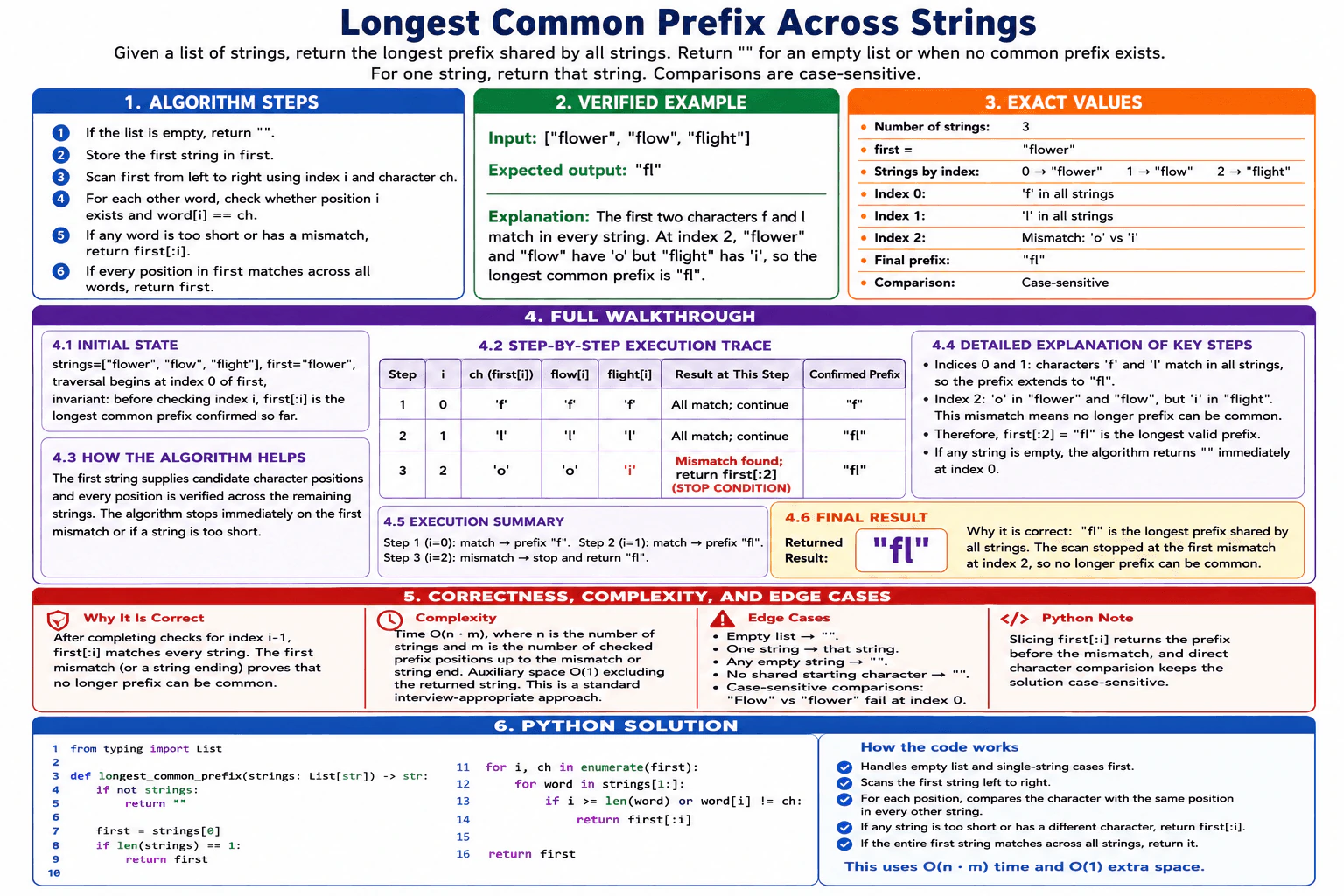
Find the common prefix across a list of strings. diagram
How to Explain It in an Interview
1. Understand the input and required output

The input is a list of strings. The output is one string containing the longest prefix shared by all strings.

For the example ["flower", "flow", "flight"], the correct output is "fl".

An empty list returns "". A list with one string returns that string. If any string is empty, the answer is "". Comparisons are case-sensitive, so uppercase and lowercase letters are different.

2. Choose vertical scanning

I use the first string as the reference. Each character position in that string is a possible position in the common prefix.

At index i, I compare first[i] with the character at index i in every other string.

The invariant is that before checking index i, first[:i] is the longest prefix confirmed to match every string so far.

3. Initialize the state

I first check whether the list is empty. If it is empty, I return "".

I then store the first string in first. If there is only one string, I return it because the whole string is its own longest common prefix.

The character scan begins at index 0 of first.

4. Walk through the example

The input is ["flower", "flow", "flight"]. The reference string is "flower".

At index 0, the reference character is 'f'. flow[0] is 'f', and flight[0] is also 'f'. All strings match, so the confirmed prefix becomes "f".

At index 1, the reference character is 'l'. flow[1] and flight[1] are also 'l'. The confirmed prefix becomes "fl".

At index 2, the reference character is 'o'. flow[2] is 'o', but flight[2] is 'i'. The condition fails because the characters are different.

The function returns first[:2], which is "fl". It stops immediately and does not process later positions.

5. Explain why the result is correct

Before index 2 is checked, the prefix first[:2], which is "fl", already matches every string.

The mismatch at index 2 proves that no prefix containing that position can be shared by all strings. Therefore, "fl" is the longest possible common prefix.

6. Explain the Python implementation

The outer loop reads the first string from left to right with enumerate(first). This gives the current index i and character ch.

The inner loop processes strings[1:], which contains every string except the reference string. For each word, the code checks whether index i exists and whether word[i] equals ch.

If the word is too short or the character is different, the function returns first[:i]. If every character in the first string matches every other string, the function returns first.

7. Explain complexity and edge cases

Let n be the number of strings. Let m be the number of positions checked before a mismatch or the end of the shortest relevant string.

The time complexity is O(n × m). At each checked position, the algorithm may compare the character with every other string. It may stop early after the first mismatch.

The shown code uses strings[1:]. That expression creates a new list containing references to the remaining strings. Its peak auxiliary space is therefore O(n). The returned prefix slice also uses space proportional to the returned prefix, but output space is usually reported separately.

Important edge cases are an empty list, one string, an empty string, no shared first character, and case-sensitive input.

Key Insight / Why This Solution Works

The key insight is to use the first string as the reference and check its characters vertically across the other strings. At each index, every string must contain the same character for the common prefix to continue. The invariant is that before checking index i, first[:i] matches every string. The first short string or mismatching character proves that no longer prefix can be common, so returning first[:i] is correct.

Code
from typing import List


def longest_common_prefix(strings: List[str]) -> str:
    # An empty list has no common prefix.
    if not strings:
        return ""

    # Use the first string as the reference string.
    first = strings[0]

    # One string is its own longest common prefix.
    if len(strings) == 1:
        return first

    # Check each character position in the first string.
    for i, ch in enumerate(first):
        # Compare this position with every remaining string.
        for word in strings[1:]:
            # Stop if the word is too short or the character differs.
            if i >= len(word) or word[i] != ch:
                return first[:i]

    # Every character in the first string matched all other strings.
    return first


if __name__ == "__main__":
    example = ["flower", "flow", "flight"]
    result = longest_common_prefix(example)
    print(result)  # fl
Time & Space Complexity

Let n be the number of strings. Let m be the number of character positions checked before the algorithm stops. For each checked position, the code may compare one character in every string, so the time complexity is O(n × m). The algorithm can stop early when it finds a mismatch. The shown code uses strings[1:], which creates a temporary list of up to n - 1 string references. Therefore, its peak auxiliary space is O(n), excluding the returned prefix.

Where it is used

This pattern is useful when several strings must be grouped or matched by their shared beginning. Examples include search suggestions, command completion, file-path grouping, dictionary prefix checks, and organizing identifiers that begin with the same characters.

Why Interviewers Ask This

This question tests careful string and index handling. The interviewer wants to see whether the candidate can choose a simple traversal order, maintain a clear invariant, stop when the result is known, and handle empty or short strings safely. It also checks whether the candidate can keep the example, code, and explanation consistent and report the real complexity of Python operations such as list slicing.

Common interview mistakes

A common mistake is reading word[i] before checking whether the word is long enough. This can cause an index error. Another mistake is returning first[:i + 1], which incorrectly includes the mismatching position. Candidates may forget the empty-list, one-string, or empty-string cases. Some continue scanning after the first mismatch even though the result is already known. Another mistake is treating uppercase and lowercase letters as equal. Candidates may also claim O(1) auxiliary space while using strings[1:], which creates a temporary list.

Interview tip

State the invariant before coding: before checking index i, first[:i] already matches every string. This makes the early return and correctness argument easy to explain.

Interviewer may ask next
How can you keep the same vertical-scanning algorithm but reduce auxiliary space?

Replace for word in strings[1:]: with an index-based loop such as for j in range(1, len(strings)): and set word = strings[j]. This avoids creating a temporary list slice. The correctness and traversal order stay the same. The time complexity remains O(n × m), while auxiliary space becomes O(1), excluding the returned prefix.

How would the solution change if comparisons should ignore letter case?

Compare normalized characters, such as word[i].lower() and ch.lower(), while still returning a prefix from the original first string. The same invariant and early-return rule remain valid because every position is still checked across all strings. The time complexity remains O(n × m). With the shown strings[1:] loop, auxiliary space remains O(n). The main tradeoff is that Unicode case conversion can have language-specific behavior.

16. Generate minimal unique word abbreviations.CodingHardApple

Question Details

Given a list of words, generate the shortest abbreviations that uniquely identify each word under the stated abbreviation rules. Explain collision handling, tie cases, unchanged words, and complexity.

Short Interview Answer (30-60 seconds)

I group words by their length, first letter, and last letter, because only words with the same signature can collide. Inside each group, I sort the words but keep their original indices. For each word, I compare it with its previous and next sorted neighbors using longest common prefix lengths. The needed prefix is one more than the larger LCP. If the abbreviation is not shorter, I keep the original word. The time is O(n log n · m), and the auxiliary space is O(n).

Detailed Explanation

See the Code while reading this explanation.

The problem asks us to create the shortest unique abbreviation for every word while preserving the original input order. An abbreviation contains a prefix, the number of omitted middle letters, and the final letter. The main challenge is handling words that would otherwise produce the same abbreviation. The diagram solves this by grouping possible collisions, sorting each group, and comparing neighboring words.

Useful Questions to Ask the Interviewer
  1. What input sizes, value ranges, and edge cases should the solution handle?
  2. What output should be returned for empty, invalid, or duplicate input?
  3. Should I prioritize execution time or memory use, and may I use the standard library?
Generate minimal unique word abbreviations. diagram
How to Explain It in an Interview
1. Group only the words that can collide

Two words can produce the same abbreviation only when they have the same length, first letter, and last letter.

I use the tuple (length, first letter, last letter) as the signature.

For the example, internal and interval share (8, i, l). The words intension and intrusion share (9, i, n). Every other word is in a singleton group.

The hash map stores:

  • Key: the signature.
  • Value: a list of (word, original_index) pairs.

The original index is saved because each group is sorted temporarily.

2. Sort each group and inspect adjacent words

I sort each signature group in lexicographic order.

After sorting, the word that shares the longest prefix with the current word must be one of its two adjacent neighbors. Therefore, I compare only the previous and next words.

This avoids comparing every word with every other word in the same group.

3. Calculate the smallest required prefix

For each word, I calculate:

  • The longest common prefix with the previous word.
  • The longest common prefix with the next word.

The required prefix length is:

1 + max(left LCP, right LCP)

For internal and interval, the shared prefix is inter, which has length 5. Both words therefore need a prefix length of 6.

For intension and intrusion, the shared prefix is int, which has length 3. Both words need a prefix length of 4.

4. Build the abbreviation or keep the word

The abbreviation contains:

  • The required prefix.
  • The number of omitted middle letters.
  • The final letter.

The omitted count is:

len(word) - prefix_len - 1

If len(word) - prefix_len <= 2, the abbreviation would not be shorter than the original word. In that case, I keep the original word.

This is why internal and interval remain unchanged. Their required prefix length is 6, so the abbreviation would not save any characters.

The pair intension and intrusion becomes inte4n and intr4n.

5. Walk through the exact example

The input is:

["like", "god", "internal", "me", "internet", "interval", "intension", "face", "intrusion"]

The execution summary is:

  • like: prefix length 1, result l2e.
  • god: prefix length 1, keep god because the abbreviation is not shorter.
  • internal: LCP 5 with interval, prefix length 6, keep internal.
  • me: prefix length 1, keep me because it is too short.
  • internet: singleton group, prefix length 1, result i6t.
  • interval: LCP 5 with internal, prefix length 6, keep interval.
  • intension: LCP 3 with intrusion, prefix length 4, result inte4n.
  • face: prefix length 1, result f2e.
  • intrusion: LCP 3 with intension, prefix length 4, result intr4n.

The final result in original order is:

["l2e", "god", "internal", "me", "i6t", "interval", "inte4n", "f2e", "intr4n"]

6. Explain why the result is correct

Only words in the same signature group can share an abbreviation.

Inside one group, sorting places words with similar prefixes next to each other. For any word, its maximum shared prefix with another word in the group is reached by its previous or next sorted neighbor. Therefore, one plus the larger neighboring LCP is the smallest prefix that separates the word from every other word in that group.

If the resulting abbreviation is not shorter, returning the original word follows the stated rule.

7. Explain the Python implementation and complexity

The code first builds the signature groups. It then sorts each group and calculates one required prefix length per word. Finally, it writes each abbreviation into the result array using the saved original index.

Let n be the number of words and m be the maximum word length. Grouping takes O(n). Sorting the groups and comparing strings takes O(n log n · m) overall. The groups, saved indices, prefix-length arrays, and result array use O(n) auxiliary space besides the returned strings.

Key Insight / Why This Solution Works

The key insight is that only words with the same length, first letter, and last letter can collide. The algorithm groups words by that signature and stores each word with its original index. It sorts each group lexicographically. In sorted order, a word's largest shared prefix with any other word is achieved by its previous or next neighbor. The required prefix is therefore one plus the larger neighboring LCP. The invariant is that each chosen prefix is the smallest prefix that makes the word unique inside its signature group. If the abbreviation is not shorter, the original word is kept.

Code
from collections import defaultdict
from typing import Dict, List, Tuple


class Solution:
    def wordsAbbreviation(self, words: List[str]) -> List[str]:
        # Create an abbreviation with the required prefix length.
        def abbreviate(word: str, prefix_len: int) -> str:
            # Keep the original word when the abbreviation is not shorter.
            if len(word) - prefix_len <= 2:
                return word

            # Count only the omitted middle letters.
            omitted = len(word) - prefix_len - 1

            # Build: prefix + omitted count + final letter.
            return f"{word[:prefix_len]}{omitted}{word[-1]}"

        # Return the length of the longest common prefix.
        def lcp(a: str, b: str) -> int:
            i = 0
            limit = min(len(a), len(b))

            # Count matching characters from the beginning.
            while i < limit and a[i] == b[i]:
                i += 1

            return i

        # Signature -> list of (word, original index).
        groups: Dict[
            Tuple[int, str, str],
            List[Tuple[str, int]],
        ] = defaultdict(list)

        # Group only words that can produce the same abbreviation.
        for index, word in enumerate(words):
            signature = (len(word), word[0], word[-1])
            groups[signature].append((word, index))

        # Results are written back using original indices.
        result = [""] * len(words)

        # Process each signature group independently.
        for group in groups.values():
            # Similar prefixes become adjacent after sorting.
            group.sort(key=lambda item: item[0])

            # A singleton group starts with a one-letter prefix.
            prefix_lengths = [1] * len(group)

            # Find the smallest prefix that separates each word.
            for i, (word, _) in enumerate(group):
                left_lcp = lcp(word, group[i - 1][0]) if i > 0 else 0
                right_lcp = lcp(word, group[i + 1][0]) if i + 1 < len(group) else 0

                prefix_lengths[i] = max(left_lcp, right_lcp) + 1

            # Build each result and restore the original input order.
            for i, (word, original_index) in enumerate(group):
                result[original_index] = abbreviate(
                    word,
                    prefix_lengths[i],
                )

        return result


if __name__ == "__main__":
    example_words = [
        "like",
        "god",
        "internal",
        "me",
        "internet",
        "interval",
        "intension",
        "face",
        "intrusion",
    ]

    answer = Solution().wordsAbbreviation(example_words)
    print(answer)
    # Expected:
    # ['l2e', 'god', 'internal', 'me', 'i6t',
    #  'interval', 'inte4n', 'f2e', 'intr4n']
Time & Space Complexity

Let n be the number of words and m be the maximum word length. Building the signature groups takes O(n). Sorting all groups takes O(n log n) comparisons in the largest case, and each string comparison may inspect up to m characters. The neighboring LCP checks also inspect at most m characters per comparison. The overall time is O(n log n · m). The groups, saved original indices, prefix-length arrays, and result array use O(n) auxiliary space besides the returned strings.

Where it is used

This pattern is useful when software needs compact but distinct names. Examples include shortened labels in a user interface, compact identifiers in reports, readable aliases for long field names, and generated labels for items with similar prefixes. The grouping and adjacent-prefix idea is also useful when many strings must be separated by the shortest distinguishing prefix.

Why Interviewers Ask This

The interviewer is checking whether you can turn a string rule into a precise grouping key and resolve collisions without comparing every pair. The problem tests sorting, longest common prefix logic, preservation of original order, and careful abbreviation arithmetic. It also shows whether you can explain why adjacent comparisons are sufficient, handle unchanged words correctly, and include string-comparison cost in the final complexity.

Common interview mistakes

Common mistakes are comparing every word with every other word, losing original indices after sorting, checking only one neighboring LCP, and forgetting that the final letter is not part of the omitted count. Another mistake is returning an abbreviation when it is not shorter than the original word. Candidates may also state O(n log n) time and forget that string comparisons can inspect up to m characters.

Interview tip

Explain the collision signature first. Then explain why sorting makes the previous and next words sufficient for the LCP check. This gives the interviewer the main correctness argument before you write the implementation.

Interviewer may ask next
Why is it enough to compare a sorted word only with its previous and next neighbors?

In lexicographic order, words with the same prefix appear together. For a current word, any word that shares its maximum prefix must be beside it on the left or right. If a non-adjacent word shared a longer prefix, the words between them would share that prefix too, so an adjacent word would be at least as similar. Therefore, the maximum neighboring LCP is sufficient. The time remains O(n log n · m), and the auxiliary space remains O(n).

How does the solution preserve the original input order after sorting each group?

Each grouped item stores both the word and its original index. Sorting changes only the temporary order inside that signature group. After calculating the prefix lengths, the algorithm writes each abbreviation into result[original_index]. This restores the exact input order. The saved indices use O(n) auxiliary space, while the overall time stays O(n log n · m).

17. Implement a FIFO queue using two stacks.CodingMediumApple

Question Details

Implement enqueue and dequeue operations for a first-in-first-out queue using two last-in-first-out stacks. Define empty behavior, amortized complexity, and edge cases.

Short Interview Answer (30-60 seconds)

I would use two stacks. New values go into in_stack. For dequeue, I first use out_stack if it already contains values. If it is empty, I move every value from in_stack to out_stack. This reverses the order, so the oldest value becomes the next one removed. An empty queue raises IndexError. Enqueue is O(1). Dequeue is amortized O(1), with O(n) worst-case time during a transfer. Auxiliary space is O(n).

Detailed Explanation

See the Code while reading this explanation.

The problem asks us to build a first-in-first-out queue using two last-in-first-out stacks. A queue removes the oldest value first, while a stack removes the newest value first. We solve this difference by using one stack for new values and another stack for values that are ready to leave. Moving values between the stacks reverses their order and restores FIFO behavior.

Useful Questions to Ask the Interviewer
  1. What input sizes, value ranges, and edge cases should the solution handle?
  2. What output should be returned for empty, invalid, or duplicate input?
  3. Should I prioritize execution time or memory use, and may I use the standard library?
Implement a FIFO queue using two stacks. diagram
How to Explain It in an Interview
1. Define the two stacks

I use in_stack and out_stack.

in_stack stores newly enqueued values. Its newest value is on top.

out_stack stores values in dequeue order. When out_stack is not empty, its top is the current front of the queue.

The stack top is the right side in list notation.

2. Implement enqueue

To enqueue a value, I append it to in_stack.

For example, after enqueue(10), enqueue(20), and enqueue(30), the state is:

in_stack = [10, 20, 30] out_stack = []

The value 30 is on top of in_stack because it is on the right.

3. Implement dequeue

For dequeue, I first check out_stack.

If out_stack already contains values, I pop its top and return it.

If out_stack is empty, I move every value from in_stack to out_stack. Each move pops from in_stack and appends to out_stack.

This reverses the order. The oldest enqueued value becomes the top of out_stack.

If out_stack is still empty after the transfer, both stacks were empty. The method raises IndexError("dequeue from empty queue").

4. Walk through the example

The operations are enqueue(10), enqueue(20), enqueue(30), dequeue(), enqueue(40), dequeue().

Step 1: enqueue(10).

Before: in_stack = [], out_stack = [].

Action: Push 10 to in_stack.

After: in_stack = [10], out_stack = [].

Step 2: enqueue(20).

Before: in_stack = [10], out_stack = [].

Action: Push 20 to in_stack.

After: in_stack = [10, 20], out_stack = [].

Step 3: enqueue(30).

Before: in_stack = [10, 20], out_stack = [].

Action: Push 30 to in_stack.

After: in_stack = [10, 20, 30], out_stack = [].

Step 4: dequeue().

Before: in_stack = [10, 20, 30], out_stack = [].

out_stack is empty, so the code transfers 30, then 20, then 10 into out_stack. The transfer produces out_stack = [30, 20, 10]. The code then pops 10.

After: in_stack = [], out_stack = [30, 20].

Returned value: 10.

Step 5: enqueue(40).

Before: in_stack = [], out_stack = [30, 20].

Action: Push 40 to in_stack.

After: in_stack = [40], out_stack = [30, 20].

Step 6: dequeue().

Before: in_stack = [40], out_stack = [30, 20].

out_stack is not empty, so no transfer is needed. The code pops 20 directly.

After: in_stack = [40], out_stack = [30].

Returned value: 20.

The returned values are [10, 20]. The remaining queue is [30, 40] from front to back.

5. Explain why the solution is correct

The central invariant is that when out_stack is not empty, its top is the oldest value currently in the queue.

Newer values stay in in_stack. When out_stack becomes empty, moving all values from in_stack reverses their order. This puts the oldest waiting value on top of out_stack.

Therefore, values leave in the same order in which they entered. That is exactly FIFO behavior.

6. Explain the Python implementation

The constructor creates two empty lists.

enqueue uses append on in_stack.

dequeue transfers values only when out_stack is empty. This avoids repeating work.

After the optional transfer, dequeue checks out_stack again. If it is still empty, the queue has no values, so the method raises IndexError.

Otherwise, it pops and returns the top value from out_stack.

7. Explain complexity and edge cases

Enqueue takes O(1) time because it performs one append.

A dequeue can take O(n) time when it transfers n values. However, each value is transferred from in_stack to out_stack at most once. Across many operations, dequeue therefore takes amortized O(1) time.

The two stacks can store up to n values in total, so auxiliary space is O(n).

Important edge cases are an empty queue, one value, many enqueues before the first dequeue, and interleaved enqueue and dequeue operations.

Key Insight / Why This Solution Works

The key idea is to split the queue state between two stacks. in_stack accepts new values in arrival order. out_stack exposes values in removal order. The central invariant is that when out_stack is not empty, its top is the current front of the queue. When out_stack is empty, moving every value from in_stack to out_stack reverses the order. The oldest waiting value then becomes the top of out_stack. We transfer only when needed, so each value is moved from in_stack to out_stack at most once. This gives the standard optimal amortized solution.

Code
class MyQueue:
    def __init__(self) -> None:
        # New values are pushed onto this stack.
        self.in_stack: list[int] = []

        # Values ready to dequeue are stored in this stack.
        self.out_stack: list[int] = []

    def enqueue(self, value: int) -> None:
        # Add the newest value to the top of in_stack.
        self.in_stack.append(value)

    def dequeue(self) -> int:
        # Transfer values only when out_stack is empty.
        if not self.out_stack:
            # Moving every value reverses the order.
            # The oldest queued value becomes the top of out_stack.
            while self.in_stack:
                self.out_stack.append(self.in_stack.pop())

        # If both stacks are empty, the queue has no value to return.
        if not self.out_stack:
            raise IndexError("dequeue from empty queue")

        # Remove and return the current front of the queue.
        return self.out_stack.pop()


if __name__ == "__main__":
    queue = MyQueue()

    # Run the same example shown in the diagram.
    queue.enqueue(10)
    queue.enqueue(20)
    queue.enqueue(30)

    first_result = queue.dequeue()

    queue.enqueue(40)

    second_result = queue.dequeue()

    # Expected output: [10, 20]
    print([first_result, second_result])

    # Final internal state shown in the diagram.
    print("in_stack:", queue.in_stack)  # [40]
    print("out_stack:", queue.out_stack)  # [30]
Time & Space Complexity

enqueue takes O(1) time because it only appends one value to in_stack. A single dequeue can take O(n) time when out_stack is empty and all n waiting values must be transferred. However, each value moves from in_stack to out_stack only once. Because of this, dequeue is amortized O(1). Amortized means the average cost across a sequence of operations is constant, even though one operation may be expensive. The two stacks hold at most n values in total, so auxiliary space is O(n).

Where it is used

This pattern is useful when queue behavior must be built from stack operations. It also teaches lazy transfer, which means delaying work until it is needed. Similar ideas appear in buffered processing and data structures that move items between internal containers to provide a different external order.

Why Interviewers Ask This

The interviewer is checking whether you can create one data structure from another while preserving its required behavior. They want to see if you understand stack order, queue order, and the effect of reversing values. They also evaluate whether you can maintain a clear invariant, handle an empty queue, avoid unnecessary transfers, write correct Python list operations, and explain the difference between worst-case O(n) time for one dequeue and amortized O(1) time across many operations.

Common interview mistakes

A common mistake is transferring values on every dequeue. The transfer should happen only when out_stack is empty. Another mistake is moving values in the wrong direction. Values must move from in_stack to out_stack. Some candidates pop from in_stack directly, which returns the newest value and breaks FIFO order. Others forget to raise an error when both stacks are empty. It is also incorrect to claim that every dequeue is always O(1). One dequeue may take O(n), while the amortized cost is O(1).

Interview tip

State the invariant before writing code: when out_stack is not empty, its top is the queue front. Then explain that a transfer happens only when out_stack is empty. This makes both correctness and the amortized O(1) dequeue cost easy to justify.

Interviewer may ask next
How would you add a peek operation that returns the front value without removing it?

peek would use the same transfer rule as dequeue. If out_stack is empty, move every value from in_stack to out_stack. If out_stack is still empty, raise IndexError because the queue is empty. Otherwise, return out_stack[-1] instead of popping it. The invariant stays the same because the top of out_stack is still the queue front. peek has amortized O(1) time, O(n) worst-case time during a transfer, and the total auxiliary space remains O(n).

Can the queue support a size operation in O(1) time?

Yes. The current number of queued values is len(in_stack) + len(out_stack). Python stores each list length, so len is O(1). The size operation returns that sum without moving any values. Correctness is preserved because every queued value is stored in exactly one of the two stacks. The operation takes O(1) time and O(1) additional space. It does not change enqueue or dequeue behavior.

18. Determine whether an undirected graph is two-colorable.CodingMediumApple

Question Details

Given an undirected graph, determine whether its nodes can be colored with two colors so that no adjacent nodes have the same color. Explain disconnected components, conflict detection, and complexity.

Short Interview Answer (30-60 seconds)

I would use BFS with a deque and a color map. The map stores each node with color 1 or -1. I loop through every node because the graph may be disconnected. For each uncolored node, I start BFS and give every uncolored neighbor the opposite color. If an edge connects two nodes with the same color, I return False immediately. If every component finishes without a conflict, I return True. The time complexity is O(V + E), and the auxiliary space is O(V).

Detailed Explanation

See the Code while reading this explanation.

The input is an undirected graph stored as an adjacency list. We must decide whether its nodes can be divided into two color groups so that every edge connects nodes from different groups. This is called checking whether the graph is bipartite, or two-colorable. BFS works well because we can color each newly discovered neighbor with the opposite color and detect a conflict immediately.

Useful Questions to Ask the Interviewer
  1. What input sizes, value ranges, and edge cases should the solution handle?
  2. What output should be returned for empty, invalid, or duplicate input?
  3. Should I prioritize execution time or memory use, and may I use the standard library?
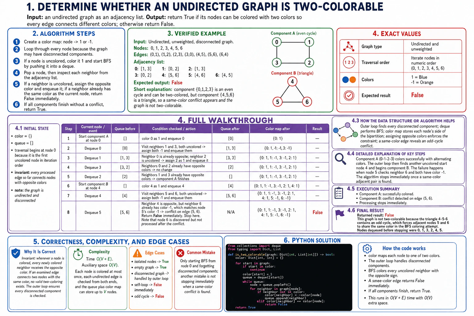
Determine whether an undirected graph is two-colorable. diagram
How to Explain It in an Interview
1. Understand the input and required output

The input is an undirected, unweighted graph represented by an adjacency list. Each dictionary key is a node. Its value is the list of nodes connected to it.

The output is a Boolean value. We return True if every connected component can be colored with two colors so that adjacent nodes have different colors. We return False when we find an edge whose two endpoints have the same color.

The graph may be disconnected. One BFS can visit only the component containing its start node, so an outer loop must check every node.

2. Choose BFS, a deque, and a color map

The color map stores node to color. Each color is either 1 or -1.

The deque is the BFS queue. It stores discovered nodes that still need to be processed.

When the current node has one color, each uncolored neighbor receives the opposite color. If a neighbor already has the same color as the current node, the graph is not two-colorable.

The central invariant is that every processed edge connects nodes with opposite colors.

3. Initialize and start each disconnected component

We begin with an empty color map.

The outer loop visits every node in the graph. If a node is already in the color map, BFS has already reached it, so we skip it.

If a node is uncolored, we start a new component. We assign it color 1 and place it in a deque.

For the diagram's example, iteration begins at node 0 because the dictionary keys are listed in numeric order.

4. Walk through the exact example

The graph has these edges:

(0,1), (1,2), (2,3), (3,0), (4,5), (5,6), and (6,4).

It contains two disconnected components.

Step 1: Start component A at node 0. The color map becomes {0: 1}. The queue becomes [0].

Step 2: Remove node 0 from the queue. Nodes 1 and 3 are uncolored, so both receive color -1. The queue becomes [1, 3]. The color map becomes {0: 1, 1: -1, 3: -1}.

Step 3: Remove node 1. Neighbor 0 already has the opposite color. Node 2 is uncolored, so it receives color 1. The queue becomes [3, 2].

Step 4: Remove node 3. Neighbors 0 and 2 already have the opposite color, so no state changes.

Step 5: Remove node 2. Neighbors 1 and 3 already have the opposite color. Component A finishes successfully.

Step 6: The outer loop reaches uncolored node 4. We assign node 4 color 1 and place it in the queue.

Step 7: Remove node 4. Nodes 5 and 6 are uncolored, so both receive color -1. The queue becomes [5, 6].

Step 8: Remove node 5. Neighbor 4 has the opposite color, which is valid. Neighbor 6 already has color -1, which is the same color as node 5. Edge (5, 6) is a conflict, so the function returns False immediately.

Node 6 was discovered and colored, but it is not removed from the queue after the conflict. The nodes removed before stopping are 0, 1, 3, 2, 4, and 5.

5. Explain why the result is correct

Whenever BFS colors a new neighbor, it assigns the negative of the current node's color. Therefore, the edge between them connects opposite colors.

If an examined edge connects two nodes with the same color, the current component cannot satisfy the two-color rule. In this example, nodes 4, 5, and 6 form a triangle. A triangle is an odd cycle, and an odd cycle cannot be colored with only two colors.

The outer loop starts BFS from every remaining uncolored node. Therefore, every disconnected component is checked.

6. Explain the Python implementation

The function creates an empty dictionary named color.

The outer for loop processes every node key. It starts BFS only when the node is not already colored.

Inside BFS, popleft removes the next node from the deque. The inner loop reads each neighbor from the adjacency list.

If a neighbor is uncolored, the code assigns -color[node] and adds the neighbor to the deque. If the neighbor already has the same color, the code returns False immediately.

If all components finish without a conflict, the function returns True.

7. Explain complexity and edge cases

The time complexity is O(V + E). V is the number of nodes, and E is the number of edges. Each node is colored at most once. Each undirected edge is examined from both endpoints, which is still O(E) total work.

The auxiliary space is O(V). The color map can store all nodes, and the deque can also contain up to V nodes.

An empty graph returns True. An isolated node is valid because it has no conflicting edge. Disconnected graphs are handled by the outer loop. A self-loop returns False because a node cannot have a different color from itself. Any odd cycle also returns False.

Key Insight / Why This Solution Works

Use BFS separately on every disconnected component. A dictionary stores each node's color as either 1 or -1. Start each uncolored component with color 1. During BFS, assign every uncolored neighbor the opposite color and add it to the deque. If an already colored neighbor has the same color as the current node, return False immediately. The invariant is that every processed edge connects nodes with opposite colors. If all components preserve this invariant, the graph is two-colorable.

Code
from collections import deque
from typing import Dict, List


def is_two_colorable(graph: Dict[int, List[int]]) -> bool:
    """Return True if the undirected graph can be colored with two colors."""

    # Map each discovered node to color 1 or -1.
    color: Dict[int, int] = {}

    # Check every node because the graph may have disconnected components.
    for start in graph:
        # This node was already reached by an earlier BFS.
        if start in color:
            continue

        # Start a new connected component with color 1.
        color[start] = 1
        queue = deque([start])

        # Process the current connected component with BFS.
        while queue:
            node = queue.popleft()

            # Check every node connected to the current node.
            for neighbor in graph[node]:
                if neighbor not in color:
                    # A newly discovered neighbor must use the opposite color.
                    color[neighbor] = -color[node]
                    queue.append(neighbor)
                elif color[neighbor] == color[node]:
                    # This edge connects equal colors, so two-coloring is impossible.
                    return False

    # Every disconnected component was colored without a conflict.
    return True


if __name__ == "__main__":
    # Exact example used in the diagram.
    example_graph: Dict[int, List[int]] = {
        0: [1, 3],
        1: [0, 2],
        2: [1, 3],
        3: [0, 2],
        4: [5, 6],
        5: [4, 6],
        6: [4, 5],
    }

    # Expected output: False.
    # Nodes 4, 5, and 6 form an odd cycle.
    print(is_two_colorable(example_graph))
Time & Space Complexity

The time complexity is O(V + E). V is the number of nodes, and E is the number of edges. Each node receives a color at most once. Each undirected edge is checked from both endpoints, so all edge checks together take O(E) time. The algorithm may stop early when it finds a conflict. The auxiliary space is O(V) because the color dictionary and the deque can each grow with the number of nodes.

Where it is used

This pattern is useful when connected items must be divided into two groups and every connection must cross between the groups. Examples include bipartite matching preparation, assigning conflicting tasks to two schedules, dividing people into two teams under opposition rules, and validating whether a relationship graph supports two compatible categories.

Why Interviewers Ask This

This problem tests whether you recognize a bipartite-graph pattern and can apply BFS correctly. The interviewer is checking whether you represent graph state clearly, color nodes at the correct time, detect a conflict early, and handle disconnected components. It also tests whether you can maintain a useful invariant, write clean deque-based Python code, and explain why the total time is O(V + E) with O(V) auxiliary space.

Common interview mistakes

A common mistake is starting BFS only from node 0, which can miss a conflicting disconnected component. Another mistake is adding a node to the queue before assigning its color, which can cause repeated discovery. Some candidates check only whether a neighbor was visited and forget to compare the two colors. Others fail to return immediately after finding a same-color edge. It is also incorrect to claim O(1) auxiliary space because the color map and deque can grow to O(V).

Interview tip

State the invariant before writing code: every processed edge must connect nodes with opposite colors. Then mention that the outer loop is required for disconnected components. These two points explain almost the entire solution.

Interviewer may ask next
How would you return the two color groups instead of only True or False?

Keep the same BFS and color map. If a conflict is found, report that no valid grouping exists. Otherwise, place every node with color 1 into one list and every node with color -1 into another list. The same invariant proves correctness because every edge still connects opposite colors. The time complexity remains O(V + E). The auxiliary space remains O(V), including the color map, queue, and returned groups. The tradeoff is that the function returns and stores more information.

Could the same check be implemented with DFS?

Yes. Keep the same color map and opposite-color rule, but use recursion or an explicit stack instead of a deque. Start DFS from every uncolored node so disconnected components are still checked. Return False when adjacent nodes have the same color. The correctness invariant remains unchanged. The time complexity is O(V + E), and the auxiliary space is O(V). Recursive DFS also uses call-stack space and may reach Python's recursion limit on a very deep graph.

19. Convert a Roman numeral to an integer.CodingEasyApple

Question Details

Given a valid Roman numeral string, return its integer value. Explain how subtractive pairs are handled, define invalid-input assumptions, and analyze time and space complexity.

Short Interview Answer (30-60 seconds)

I scan the Roman numeral from right to left and use a fixed lookup map for the seven Roman symbols. I keep a running total and the value of the symbol immediately to the right. If the current value is smaller than that previous value, I subtract it. Otherwise, I add it. This handles pairs such as IV, XC, and CM correctly. The solution takes O(n) time and O(1) auxiliary space because the lookup map has a fixed size.

Detailed Explanation

See the Code while reading this explanation.

The input is a valid Roman numeral string, and the output is its integer value. I scan from right to left because this makes subtractive pairs easy to detect. When the current symbol is smaller than the symbol immediately to its right, I subtract it. Otherwise, I add it.

Useful Questions to Ask the Interviewer
  1. What input sizes, value ranges, and edge cases should the solution handle?
  2. What output should be returned for empty, invalid, or duplicate input?
  3. Should I prioritize execution time or memory use, and may I use the standard library?
Convert a Roman numeral to an integer. diagram
How to Explain It in an Interview
1. Understand the input and output

The function receives a valid Roman numeral string such as "MCMXCIV". It must return the integer 1994.

The question guarantees that the Roman numeral is valid. Therefore, this solution does not need to reject invalid formats.

The symbol values are I = 1, V = 5, X = 10, L = 50, C = 100, D = 500, and M = 1000.

2. Choose the algorithm and lookup map

I use a fixed lookup map from each Roman symbol to its integer value.

I scan the string from right to left. I keep two variables:

total stores the value calculated so far.

prev_value stores the value of the symbol immediately to the right of the next symbol being processed.

If current_value < prev_value, the current symbol is part of a subtractive pair, so I subtract it. Otherwise, I add it.

The invariant is that before each new character is processed, total equals the value of the suffix already processed, and prev_value equals the value of that suffix's leftmost symbol, which is immediately to the right of the next character.

3. Initialize the state

Set total = 0 and prev_value = 0.

The scan starts at the rightmost character. Every Roman symbol has a positive value, so the first value is added because it is greater than or equal to zero.

4. Walk through the example

The example is MCMXCIV, with indices 0 through 6.

At index 6, the character is V and its value is 5. The previous value is 0. Since 5 is greater than or equal to 0, add 5. The state becomes total = 5 and prev_value = 5.

At index 5, the character is I and its value is 1. Since 1 is smaller than 5, subtract 1. The state becomes total = 4 and prev_value = 1. This is how IV contributes 4.

At index 4, the character is C and its value is 100. Since 100 is greater than or equal to 1, add 100. The state becomes total = 104 and prev_value = 100.

At index 3, the character is X and its value is 10. Since 10 is smaller than 100, subtract 10. The state becomes total = 94 and prev_value = 10. This handles XC.

At index 2, the character is M and its value is 1000. Since 1000 is greater than or equal to 10, add 1000. The state becomes total = 1094 and prev_value = 1000.

At index 1, the character is C and its value is 100. Since 100 is smaller than 1000, subtract 100. The state becomes total = 994 and prev_value = 100. This handles CM.

At index 0, the character is M and its value is 1000. Since 1000 is greater than or equal to 100, add 1000. The state becomes total = 1994 and prev_value = 1000.

All seven characters have now been processed. The function returns 1994.

5. Explain why the result is correct

Roman numeral values are normally added. A smaller symbol that appears immediately before a larger symbol must be subtracted.

Scanning from right to left lets the algorithm compare each symbol with the symbol immediately to its right. The algorithm subtracts exactly when the current value is smaller. In every other case, it adds. Therefore, after every step, total remains equal to the value of the suffix already processed.

6. Explain the Python implementation

The dictionary maps each Roman character to its integer value. The loop uses reversed(s) to visit the string from right to left.

For each character, the code reads current_value. It compares that value with prev_value, adds or subtracts it, and then updates prev_value.

After the loop finishes, total contains the full integer value and is returned.

7. Explain complexity and edge cases

The algorithm processes each of the n characters once, so the time complexity is O(n).

The lookup map always contains seven entries. The other state consists of two integer variables. Therefore, the auxiliary space complexity is O(1).

Relevant cases include a single symbol such as V, repeated symbols such as III, and valid subtractive pairs such as IV, IX, XL, XC, CD, and CM. Invalid-format validation is outside this solution because the input is guaranteed to be valid.

Key Insight / Why This Solution Works

The key insight is to scan from right to left. This makes the symbol immediately to the right available through prev_value. A fixed lookup map converts each Roman character to its integer value. The invariant is that total equals the value of the suffix already processed. If the current value is smaller than prev_value, Roman numeral rules require subtraction. Otherwise, the value is added. Updating prev_value after every character keeps the comparison correct for the next step.

Code
class Solution:
    def romanToInt(self, s: str) -> int:
        # Map every Roman numeral symbol to its integer value.
        values = {
            "I": 1,
            "V": 5,
            "X": 10,
            "L": 50,
            "C": 100,
            "D": 500,
            "M": 1000,
        }

        # Store the value calculated from the processed suffix.
        total = 0

        # Store the value of the symbol immediately to the right.
        prev_value = 0

        # Process the Roman numeral from right to left.
        for ch in reversed(s):
            # Look up the integer value of the current symbol.
            current_value = values[ch]

            # A smaller value before a larger value must be subtracted.
            if current_value < prev_value:
                total -= current_value
            else:
                total += current_value

            # Save this value for the next comparison.
            prev_value = current_value

        # Return the completed integer value.
        return total


if __name__ == "__main__":
    roman = "MCMXCIV"
    result = Solution().romanToInt(roman)
    print(result)  # 1994
Time & Space Complexity

Let n be the number of characters in the Roman numeral. The loop processes every character once, so the time complexity is O(n). The lookup map always has the same seven entries, and the algorithm uses only total, prev_value, and current_value. Its memory use does not grow with n. Therefore, the auxiliary space complexity is O(1).

Where it is used

This pattern is useful when the meaning of one item depends on the item immediately after it. Scanning in reverse can remove the need for complicated look-ahead logic. Similar ideas appear in parsers, encoded-value readers, and string-processing tasks where a symbol changes meaning based on its right-side neighbor.

Why Interviewers Ask This

This problem checks whether the candidate can turn a written rule into a simple algorithm. The interviewer is evaluating traversal choice, state management, handling of subtractive pairs, and consistency between the explanation and code. It also tests whether the candidate can maintain an invariant, trace an example accurately, write clear Python, respect the valid-input assumption, and report the correct O(n) time and O(1) auxiliary space complexity.

Common interview mistakes

A common mistake is comparing the current symbol with the wrong neighbor. Another mistake is forgetting to update prev_value after each character. Some candidates subtract a symbol because it is smaller than any later symbol, but this method compares it with the symbol immediately to its right. Another mistake is changing the traversal direction without changing the comparison logic. Candidates may also claim O(n) extra space because a dictionary is used, but this dictionary always has seven entries, so the auxiliary space is O(1).

Interview tip

State the invariant before writing the loop: total is the value of the suffix already processed, and prev_value is the value immediately to the right of the next character. This makes the subtraction rule easy to explain.

Interviewer may ask next
How would you change the solution if invalid Roman numeral strings had to be rejected?

I would keep the same conversion logic but add validation for legal symbols, repetition limits, ordering rules, and allowed subtractive pairs such as IV, IX, XL, XC, CD, and CM. Invalid forms such as IL or repeated V would be rejected. Validation and conversion would still take O(n) time and O(1) auxiliary space because the Roman numeral rule set is fixed. The tradeoff is more code and more cases to test.

Can the same conversion be done by scanning from left to right?

Yes. Compare each current value with the next value. If the current value is smaller, subtract it. Otherwise, add it. The last symbol must also be added, either after the loop or through a boundary condition. Correctness is preserved because the decision still uses the immediate right-side neighbor. The complexity remains O(n) time and O(1) auxiliary space. The tradeoff is that the code needs explicit look-ahead logic.

20. Write a program to output all prime numbers up to n.CodingEasyApple

Question Details

Given an integer n, return or print all prime numbers from 2 through n. Define behavior for n below 2, explain the primality approach, and analyze time and space complexity.

Short Interview Answer (30-60 seconds)

I would use the Sieve of Eratosthenes. I create a boolean array where each index represents the same number. I mark 0 and 1 as not prime. Then I process possible base primes starting from 2. For each confirmed prime p, I mark its multiples from p squared as composite. I stop when p squared is greater than n. The remaining True indices are the primes. The time complexity is O(n log log n), and the auxiliary space complexity is O(n).

Detailed Explanation

See the Code while reading this explanation.

The problem asks us to return every prime number from 2 through n. If n is less than 2, we return an empty list. The Sieve of Eratosthenes is a good fit because it finds all primes in the range together. It removes composite numbers by marking multiples of confirmed primes.

Useful Questions to Ask the Interviewer
  1. What input sizes, value ranges, and edge cases should the solution handle?
  2. What output should be returned for empty, invalid, or duplicate input?
  3. Should I prioritize execution time or memory use, and may I use the standard library?
Write a program to output all prime numbers up to n. diagram
How to Explain It in an Interview
1. Understand the input and required output

The input is one integer named n. The output is a list containing every prime number from 2 through n in ascending order.

A prime number has exactly two positive factors: 1 and itself. If n is less than 2, there are no prime numbers in the range, so the function returns an empty list.

For the example n = 20, the output is [2, 3, 5, 7, 11, 13, 17, 19].

2. Choose the algorithm and data structure

I use the Sieve of Eratosthenes and a boolean array named is_prime. Each array index represents the number with the same value. For example, is_prime[7] tells us whether 7 is still considered prime.

The central invariant is: any value already marked False has a smaller prime factor. Therefore, that value is composite.

This method is more suitable than checking every number separately when we need all primes up to the same limit.

3. Initialize the state

I create is_prime with n + 1 entries and set every entry to True. The valid indices are 0 through n.

I then set is_prime[0] and is_prime[1] to False because 0 and 1 are not prime.

The variable p starts at 2. The loop continues while p * p <= n.

4. Walk through the example n = 20

The array covers indices 0 through 20. Indices 0 and 1 are False. Indices 2 through 20 begin as True.

For p = 2, the condition 2 * 2 <= 20 is true, and is_prime[2] is True. I start at 2 squared, which is 4. I mark 4, 6, 8, 10, 12, 14, 16, 18, and 20 as False. The values still marked True are 2, 3, 5, 7, 9, 11, 13, 15, 17, and 19.

For p = 3, the condition 3 * 3 <= 20 is true, and is_prime[3] is True. I start at 3 squared, which is 9. I mark 9, 12, 15, and 18 as False. The values still marked True are 2, 3, 5, 7, 11, 13, 17, and 19.

For p = 4, the condition 4 * 4 <= 20 is true, but is_prime[4] is False. I skip the marking step because 4 is already known to be composite. The state does not change.

The next value is p = 5. Now 5 * 5 is 25, which is greater than 20. The loop stops. I collect every index from 2 through 20 whose value is still True. The returned result is [2, 3, 5, 7, 11, 13, 17, 19].

5. Explain why the result is correct

Every composite number up to n has at least one prime factor no greater than the square root of n.

For each confirmed prime p, the algorithm marks its composite multiples. It starts at p squared because every smaller multiple of p already has a smaller prime factor and was handled earlier.

After all required base values have been processed, every composite number is False. Therefore, every index that remains True is prime.

6. Explain the Python implementation

The function first handles the n < 2 case. It then creates the is_prime array and marks indices 0 and 1 as False.

A while loop processes p while p * p <= n. If is_prime[p] is True, a for loop marks multiples from p * p through n. The loop uses a step of p. After each outer-loop iteration, p increases by 1.

Finally, a list comprehension returns every index from 2 through n whose entry is still True.

7. Explain complexity and edge cases

The time complexity is O(n log log n). The sieve marks multiples of primes in an efficient combined process.

The auxiliary space complexity is O(n) because the boolean array contains n + 1 entries.

Important edge cases are n < 2, which returns []; n = 2, which returns [2]; and small limits such as 3 or 4. The result stays in ascending order because the final list scans indices from 2 to n.

Key Insight / Why This Solution Works

The key idea is to mark composite numbers instead of testing every number independently. The algorithm creates a boolean array where index i represents the number i. It initially treats every number as a possible prime, except 0 and 1. For each confirmed prime p, it marks multiples from p squared as False. Starting at p squared avoids repeated work because smaller multiples already have smaller prime factors. The invariant is that every value marked False has a discovered smaller prime factor. After processing base values up to the square root of n, the indices still marked True are exactly the prime numbers.

Code
from typing import List


def primes_up_to(n: int) -> List[int]:
    # No prime numbers exist below 2.
    if n < 2:
        return []

    # Each index represents the number with the same value.
    # Start by treating every number as a possible prime.
    is_prime = [True] * (n + 1)

    # Zero and one are not prime numbers.
    is_prime[0] = False
    is_prime[1] = False

    # Process possible base primes starting from 2.
    p = 2
    while p * p <= n:
        # A True entry means p is a confirmed prime.
        if is_prime[p]:
            # Start at p squared because smaller multiples
            # were already handled by smaller prime factors.
            for multiple in range(p * p, n + 1, p):
                is_prime[multiple] = False

        # Move to the next possible base value.
        p += 1

    # Return every number that is still marked as prime.
    return [i for i in range(2, n + 1) if is_prime[i]]


if __name__ == "__main__":
    example_n = 20
    result = primes_up_to(example_n)
    print(result)
    # Expected output: [2, 3, 5, 7, 11, 13, 17, 19]
Time & Space Complexity

The time complexity is O(n log log n). The sieve reaches this time by marking multiples of each prime instead of checking every number with repeated division. The auxiliary space complexity is O(n). Auxiliary space means the extra memory used by the algorithm. The is_prime array contains n + 1 boolean entries, so its size grows in direct proportion to n.

Where it is used

The Sieve of Eratosthenes is useful when a program needs all prime numbers up to a known limit. It can be used in number-theory programs, factorization helpers, competitive-programming problems, and systems that answer many prime-related queries over the same range. It is more efficient than testing every value separately when the full prime list is required.

Why Interviewers Ask This

The interviewer is checking whether you recognize that the task asks for every prime in a range and select the Sieve of Eratosthenes. They also want to see whether you can map numbers to boolean-array indices, maintain the composite-marking invariant, use p squared as the starting point, stop at the square-root boundary, handle small inputs, write correct Python, and explain O(n log log n) time with O(n) auxiliary space.

Common interview mistakes

A common mistake is treating 0 or 1 as prime. Another mistake is using range(p * p, n, p), which fails to mark n when n is a multiple of p. Some candidates start at 2 * p instead of p * p. That can still produce the correct result, but it repeats work already done by smaller primes. Another mistake is using the wrong stopping condition instead of p * p <= n. It is also incorrect to claim O(n) time or O(1) auxiliary space for this implementation.

Interview tip

Explain why marking starts at p squared. Say that every smaller multiple of p already has a smaller prime factor and was handled earlier. This shows that you understand both the correctness and the efficiency of the sieve.

Interviewer may ask next
How would you handle a very large value of n when the full boolean array uses too much memory?

I would use a segmented sieve. First, I would generate the base primes up to sqrt(n). Then I would divide the range into smaller blocks and mark composites inside one block at a time. Correctness is preserved because every composite still has a prime factor no greater than sqrt(n). The total time remains about O(n log log n). Working memory depends on the block size plus the base-prime list. The tradeoff is more complex code.

What would you do if you only needed to test whether one number is prime?

A full sieve would usually be unnecessary. I would test possible divisors from 2 through the square root of that number and stop if one divides it evenly. This works because every composite number has a factor no greater than its square root. The time complexity is O(sqrt(n)), and the auxiliary space complexity is O(1). The tradeoff is that this method is less efficient when many numbers in the same range must be checked.

More questions load as you scroll

Disclaimer: This interview guide is for educational and informational purposes only. It is designed to help readers prepare, but it does not guarantee any interview result, hiring decision, offer, or outcome. Interview questions, hiring criteria, and preferred answers can vary by employer, interviewer, industry, location, and time. The examples and explanations reflect the authors' research and judgment, are provided without warranties of any kind, and should not be treated as the only correct approach. Diagrams are simplified illustrations intended to highlight the main components and their interactions; actual systems and implementations may be more complex. Alternative approaches may be equally valid or better suited to a particular question, context, or interviewer. To the fullest extent permitted by applicable law, the author, contributors, and publisher are not liable for decisions made, actions taken, or losses incurred based on this guide.

Company Notice: This guide is an independent educational resource and is not affiliated with, endorsed by, sponsored by, or approved by the company named in this guide. Company names are used only to identify interview experiences commonly reported by candidates. Interview practices can change without notice, and inclusion of company-specific content does not mean these questions are official, complete, or guaranteed to be asked. To the fullest extent permitted by law, the author, contributors, and publisher are not responsible for outcomes related to use of this material.