Meta Python Developer Interview Questions & Answers

I would use breadth-first search with a deque. I process the tree one level at a time from left to right. At each level, I append the value of the last node removed from the queue because that node is visible from the right side. I add each node’s left child before its right child. Every node is enqueued and dequeued once, so the time complexity is O(n). The auxiliary space is O(w), where w is the maximum tree width.

The input is the root of a binary tree. We must return one node value from each level, representing what is visible from the right side. Breadth-first search fits this problem because it naturally visits the tree level by level. By processing each level from left to right, the last node processed at that level is the visible node.

1. What input sizes, value ranges, and edge cases should the solution handle?
2. What output should be returned for empty, invalid, or duplicate input?
3. Should I prioritize execution time or memory use, and may I use the standard library?

The input is a reference to the root of a binary tree. The tree is not assumed to be a binary search tree.

The output is a list of node values. It contains one visible value from every level, ordered from the root level to the deepest level.

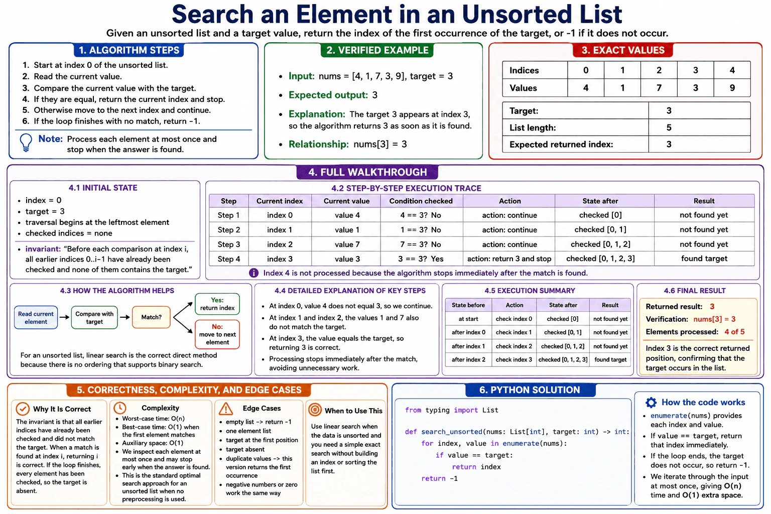
For the displayed tree, the levels are [1], [2, 3], [4, 5, 7], and [6]. The returned right-side view is [1, 3, 7, 6].

I use breadth-first search, also called BFS. BFS processes the tree one level at a time.

A deque stores nodes that are waiting to be processed. It supports efficient removal from the front and insertion at the back.

The central rule is that nodes in each level are processed from left to right. Therefore, the final node removed at that level is the rightmost visible node.

I create an empty list named result.

If root is None, the tree is empty, so I return result immediately.

Otherwise, I place the root in the deque. For the example, the initial queue is [1], and the initial result is [].

At level 0, the queue is [1]. The level size is 1. I remove node 1. It is the last node in this level, so I append 1. I then add its left child 2 and right child 3. The result is [1].

At level 1, the queue is [2, 3]. The level size is 2. I remove node 2 and add its children 4 and 5. I then remove node 3. It is the last node in the level, so I append 3. I add its right child 7. The result is [1, 3].

At level 2, the queue is [4, 5, 7]. The level size is 3. I process node 4, then node 5, then node 7. Node 5 adds its left child 6. Node 7 is the last node in this level, so I append 7. The result is [1, 3, 7].

At level 3, the queue is [6]. The level size is 1. I remove node 6. It is the last node in the level, so I append 6. The result becomes [1, 3, 7, 6].

The queue is now empty, so the traversal stops and the function returns [1, 3, 7, 6].

At the start of each outer-loop iteration, the queue contains the nodes of the next level in left-to-right order.

The inner loop removes exactly those nodes. Because the final removed node is the rightmost node in that level, appending its value records the correct visible value.

Repeating this for every level produces the complete right-side view from top to bottom.

The outer while loop continues while the deque contains nodes.

At the start of a level, level_size stores the current queue length. This separates the current level from children added for the next level.

The inner loop removes exactly level_size nodes. When i equals level_size - 1, the current node is the final node in that level, so its value is appended to result.

The code adds the left child before the right child. This preserves left-to-right processing order.

The time complexity is O(n), where n is the number of nodes. Every node is added to the deque once and removed once.

The auxiliary space complexity is O(w), where w is the maximum number of nodes stored in the queue at one level.

An empty tree returns []. A tree with one node returns [root.val]. In a left-skewed or right-skewed tree, every node appears in the result because each level contains one node.

The key insight is to process the binary tree level by level with BFS. A deque stores the nodes waiting to be visited. At the beginning of each level, its current length gives the number of nodes that belong to that level. The algorithm removes those nodes from left to right and records the value of the final removed node. The invariant is that the queue presents each current level in left-to-right order, so its last processed node is exactly the node visible from the right side.

The time complexity is O(n), where n is the total number of nodes. Each node enters the deque once and leaves it once. The auxiliary space complexity is O(w), where w is the maximum number of nodes stored in the queue at one level. A wide tree may therefore use more queue memory than a narrow tree.

A candidate may record the first node at each level, which produces the left-side view. Another mistake is to let the inner loop use a changing queue length instead of saving level_size first. Some candidates add right children before left children but still record the final node, which changes the meaning of the invariant. Using list.pop(0) instead of deque.popleft() makes front removal slower. It is also incorrect to assume that the input follows binary search tree ordering.

State the invariant before writing code: because each level is processed from left to right, the last node removed from that level is the node visible from the right side.

I would use Python’s OrderedDict to store each key-value pair and track its usage order. The leftmost key is the least recently used, and the rightmost key is the most recently used. On a successful get, I move the key to the right end and return its value. On put, I insert or update the key, move it to the right end, and remove the leftmost key if capacity is exceeded. Both operations take O(1) average time, with O(capacity) auxiliary space.

The problem asks us to build a cache with a fixed capacity. get(key) must return the stored value or -1. put(key, value) must insert or update a key. When the cache becomes too large, it must remove the least recently used key. Python’s OrderedDict fits because it stores key-value pairs in order and supports moving and removing entries in O(1) average time.

1. What input sizes, value ranges, and edge cases should the solution handle?
2. What output should be returned for empty, invalid, or duplicate input?
3. Should I prioritize execution time or memory use, and may I use the standard library?

The cache stores at most capacity entries.

get(key) returns the stored value when the key exists. It returns -1 when the key is missing.

put(key, value) inserts a new key or updates an existing key. It returns None. If the cache size becomes greater than capacity, it removes the least recently used key.

The OrderedDict stores key to value pairs.

Its order represents usage order. The leftmost entry is the least recently used entry. The rightmost entry is the most recently used entry.

The main invariant is that each cached key appears exactly once, and the dictionary order is always LRU to MRU.

First, check whether the key exists.

If it is missing, return -1. The cache order stays unchanged.

If it exists, call move_to_end(key). This moves the key to the right end, so it becomes the most recently used key. Then return its stored value.

If the key already exists, move it to the right end. Then store the new value.

If the key is new, assigning the value inserts it at the right end.

After the assignment, compare the cache size with capacity. If the size is too large, call popitem(last=False). The argument last=False removes the leftmost entry, which is the least recently used entry.

The capacity is 3.

Start with an empty cache: {}.

put(1,10) gives {1:10}.

put(2,20) gives {1:10, 2:20}.

put(3,30) gives {1:10, 2:20, 3:30}.

get(2) returns 20. Key 2 moves to the MRU position. The order becomes {1:10, 3:30, 2:20}.

put(4,40) first creates four entries. Key 1 is the leftmost and least recently used key, so it is removed. The cache becomes {3:30, 2:20, 4:40}.

get(1) returns -1 because key 1 is no longer present. The state remains {3:30, 2:20, 4:40}.

The final LRU-to-MRU key order is [3, 2, 4]. The final MRU-to-LRU key order is [4, 2, 3].

Every successful get moves its key to the right end. Every put also places its key at the right end. Therefore, the rightmost key is always the most recently used key.

The leftmost key is the key that has gone the longest without being accessed or updated. When the cache exceeds capacity, removing the leftmost entry removes exactly the least recently used key.

OrderedDict lookup, assignment, move_to_end, and popitem take O(1) average time. Therefore, get and put each take O(1) average time.

The cache stores at most capacity entries, so the auxiliary space is O(capacity).

Important cases include a missing key, updating an existing key, capacity 1, and repeated gets on the same key.

The key insight is to store both values and recency order in one OrderedDict. The central invariant is that entries are ordered from LRU on the left to MRU on the right. A successful get moves its key to the right end. A put inserts or updates a key and also places it at the right end. If the size exceeds capacity, removing the leftmost entry evicts exactly the least recently used key. This is more suitable than a plain dictionary because OrderedDict directly supports moving a key and removing the oldest entry in O(1) average time.

Each get operation takes O(1) average time. It performs an OrderedDict lookup and may move one key to the end. Each put operation also takes O(1) average time. It assigns one value, may move one key, and may remove one leftmost entry. These OrderedDict operations are constant time on average, not guaranteed constant time in every worst case. The cache stores at most capacity entries, so the auxiliary space is O(capacity).

A common mistake is returning a value without moving the accessed key to the MRU position. Another mistake is evicting the rightmost key instead of the leftmost key. Some candidates remove an entry before the cache size actually exceeds capacity. Others forget that updating an existing key must also make it most recently used. It is also incorrect to claim guaranteed O(1) worst-case time because OrderedDict operations are O(1) on average.

State the invariant before writing code: the leftmost entry is LRU, and the rightmost entry is MRU. Then explain each operation using that rule. A successful get moves right, a put places the key right, and overflow removes one key from the left.

I track the lowest price seen so far and the best profit found so far. I process the prices from left to right. For each price, I update the running minimum, calculate the profit from selling at the current price, and keep the larger profit. This preserves the buy-before-sell rule because the minimum comes only from processed days. The algorithm takes O(n) time and uses O(1) auxiliary space.

The input is a list of daily stock prices. We need the largest profit from one buy followed by one sell. If no profitable trade exists, we return 0. The best approach is to track the cheapest price seen so far and treat each current price as a possible selling price. This avoids checking every possible pair.

1. What input sizes, value ranges, and edge cases should the solution handle?
2. What output should be returned for empty, invalid, or duplicate input?
3. Should I prioritize execution time or memory use, and may I use the standard library?

Each list value is a stock price, and its index represents the day.

We must buy before we sell. The function returns the maximum profit, not the buy and sell indices.

For [7, 1, 5, 3, 6, 4], the best trade is:

• Buy at price 1, which is at index 1.
• Sell at price 6, which is at index 4.
• Profit is 6 - 1 = 5.

The returned result is 5.

I use two main variables:

• min_price stores the cheapest price seen so far.
• max_profit stores the largest valid profit found so far.

The invariant is that after processing index i, min_price is the minimum price in prices[0..i], and max_profit is the best one-transaction profit that can be made using the processed days.

A brute-force solution would compare every possible buy and sell pair. That takes O(n²) time. The running-minimum approach takes O(n) time.

Set min_price to infinity. This allows the first real price to become the first running minimum.

Set max_profit to 0. This is correct when prices only decrease because making no profitable trade should return 0.

Traversal begins at index 0.

At index 0, the price is 7.

• Minimum before: infinity.
• Update min_price to 7.
• Current profit: 7 - 7 = 0.
• Best profit remains 0.

At index 1, the price is 1.

• Minimum before: 7.
• Update min_price to 1.
• Current profit: 1 - 1 = 0.
• Best profit remains 0.

At index 2, the price is 5.

• The running minimum remains 1.
• Current profit: 5 - 1 = 4.
• Update the best profit to 4.

At index 3, the price is 3.

• The running minimum remains 1.
• Current profit: 3 - 1 = 2.
• This does not beat 4, so the best profit remains 4.

At index 4, the price is 6.

• The running minimum remains 1.
• Current profit: 6 - 1 = 5.
• Update the best profit to 5.

At index 5, the price is 4.

• The running minimum remains 1.
• Current profit: 4 - 1 = 3.
• This does not beat 5.

All six prices are processed. The function returns 5.

For each possible selling day, min_price represents the cheapest buying price from the processed days.

The algorithm calculates the profit from selling on the current day after using that running minimum. A positive profit can only come from a lower price on an earlier day. Therefore, it never uses a future price as the buy price.

Because every day is considered as a possible selling day and max_profit keeps the largest valid result, the final answer is the maximum one-transaction profit.

The loop visits prices from left to right.

First, it updates min_price with the current price. Next, it calculates current_profit by subtracting min_price from the current price. Then it updates max_profit if the current profit is larger.

After all prices are processed, the function returns max_profit.

The loop processes each price once, so the time complexity is O(n).

The algorithm stores only a few variables, so the auxiliary space complexity is O(1).

An empty list or a list with one price returns 0. A strictly decreasing list also returns 0. Equal and repeated prices are handled correctly.

The key insight is to treat every current price as a possible selling price. To find the best profit for that day, we only need the cheapest price seen so far. The algorithm keeps that value in min_price and keeps the largest calculated profit in max_profit. The invariant is that after processing index i, min_price is the minimum value in prices[0..i], and max_profit is the best valid one-buy, one-sell profit from the processed days. This produces the same result as checking all pairs but reduces the time from O(n²) to O(n).

The time complexity is O(n), where n is the number of prices. The loop processes each price once. The auxiliary space complexity is O(1) because the algorithm uses only min_price, current_profit, and max_profit. The amount of extra memory does not grow when the input becomes larger.

A common mistake is using a future price as the buying price. The running minimum must contain only the current and earlier processed prices. Another mistake is returning a negative profit when all prices decrease instead of keeping the answer at 0. Some candidates confuse the prices 1 and 6 with their indices 1 and 4. Others use nested loops and produce an unnecessary O(n²) solution. It is also incorrect to reset the best profit when a later current profit is smaller.

Explain the invariant before coding: min_price is the cheapest processed price, and max_profit is the best valid profit from the processed days. Then make each code line match that invariant.

I first handle the empty-list case by returning 0.0. For a non-empty list, I keep a running total and add each book price to it. After processing every price, I divide the total by the number of prices. For [10.0, 20.5, 15.5, 30.0], the total is 76.0 and the average is 19.0. This is correct because an arithmetic mean is the sum divided by the count. The time complexity is O(n), and the auxiliary space complexity is O(1).

The problem gives a list of book prices and asks for their arithmetic mean. Arithmetic mean means the total of all prices divided by the number of prices. A running total is enough, so we can solve the problem with one loop and constant extra memory. We must check for an empty list first because dividing by zero is invalid.

1. What input sizes, value ranges, and edge cases should the solution handle?
2. What output should be returned for empty, invalid, or duplicate input?
3. Should I prioritize execution time or memory use, and may I use the standard library?

The input is a list of book prices. The function returns one floating-point value.

For a non-empty list, the returned value is:

sum of all prices / number of prices

For an empty list, the required result is 0.0.

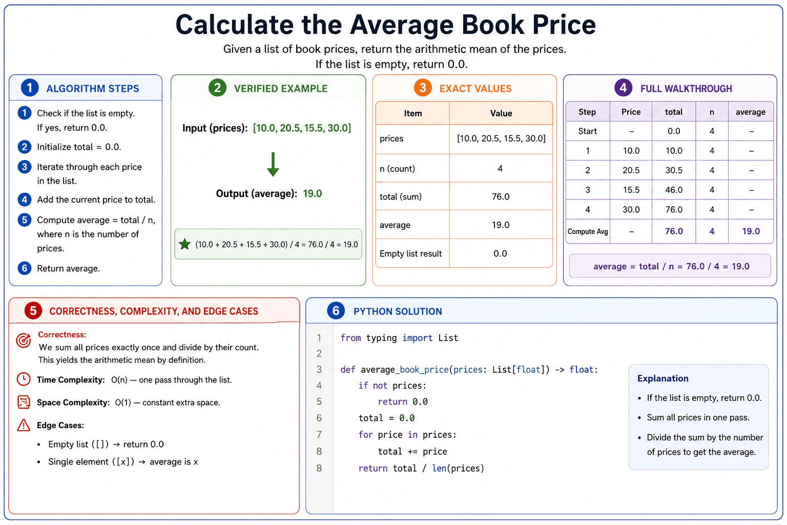
The diagram uses this example:

prices = [10.0, 20.5, 15.5, 30.0]

The expected result is 19.0.

First, check whether prices is empty. If it is empty, return 0.0 immediately.

For a non-empty list, initialize total to 0.0. The variable total stores the sum of all prices processed so far.

The central invariant is simple: after each loop iteration, total equals the sum of every price already processed.

Start with:

total = 0.0

Process the values from left to right.

Add 10.0. The total changes from 0.0 to 10.0.

Add 20.5. The total changes from 10.0 to 30.5.

Add 15.5. The total changes from 30.5 to 46.0.

Add 30.0. The total changes from 46.0 to 76.0.

After the loop, all four prices have been processed.

The final total is 76.0. The number of prices is 4.

average = total / count

average = 76.0 / 4

average = 19.0

The function returns 19.0.

At the start, total is 0.0, which is the sum of zero processed prices.

Each loop iteration adds the current price to total. Therefore, the invariant remains true after every iteration.

When the loop finishes, total is the sum of the full list. Dividing that sum by the list length gives the arithmetic mean by definition.

The condition if not prices handles the empty-list case and prevents division by zero.

The variable total begins at 0.0. The for loop adds each price to it. After the loop, len(prices) gives the count. The function returns total / len(prices).

Let n be the number of prices. The loop processes all n prices once, so the time complexity is O(n).

The function uses only the running total and normal local variables. Its auxiliary space complexity is O(1).

For an empty list, it returns 0.0. For a list containing one value, the average is that value.

Use a running sum. Begin with total = 0.0, then add each price to it. The invariant is that total always equals the sum of all prices processed so far. When the loop ends, total is the sum of the complete list. Dividing it by len(prices) gives the arithmetic mean. This approach directly follows the definition of average and does not need an additional data structure.

Let n be the number of book prices. The loop visits each of the n prices once, so the time complexity is O(n). The function keeps only a running total and a few local values. This extra memory does not grow when the input grows, so the auxiliary space complexity is O(1).

A common mistake is forgetting the empty-list check, which can cause division by zero. Another mistake is dividing during each loop iteration instead of waiting until the complete total is known. Candidates may also divide by the wrong count, return the sum instead of the average, or claim O(1) time even though every input price must be processed.

Explain the invariant before coding: after each iteration, total is the sum of all prices processed so far. This makes the loop and the correctness argument easy to follow.

I use a stack to build the canonical path. I split the absolute path by "/" and process each token from left to right. I ignore empty tokens and ".". For "..", I pop one directory only when the stack is not empty. Every normal directory name is pushed onto the stack. Finally, I join the stack with "/" and add one leading slash. This takes O(n) time and uses O(n) auxiliary space.

The problem asks us to simplify an absolute Unix-style path. We must remove repeated separators, ignore ".", and process ".." as moving to the parent directory. A stack fits this problem because it stores the valid path from the root to the current location.

1. What input sizes, value ranges, and edge cases should the solution handle?
2. What output should be returned for empty, invalid, or duplicate input?
3. Should I prioritize execution time or memory use, and may I use the standard library?

The input is an absolute Unix-style path. It starts at the root directory.

We must return its canonical form. The result has one leading slash. It has no repeated separators, no trailing slash unless the result is the root, and no special "." or ".." components.

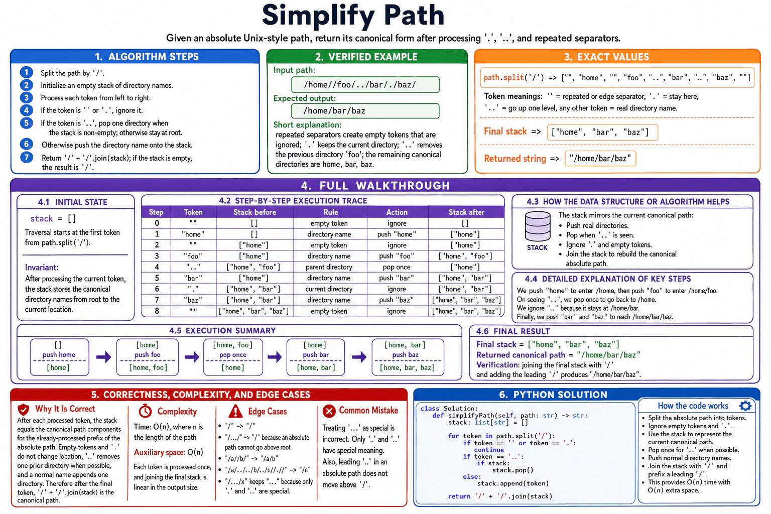
For the example input "/home//foo/../bar/./baz/", the expected output is "/home/bar/baz".

The stack stores the directory names in the current canonical path.

Each stack entry is one real directory name. The bottom entry is closest to the root. The top entry is the current directory.

The central invariant is: after each token is processed, the stack contains the canonical directory names for the processed part of the path.

Start with an empty stack.

Split the path by "/". The example produces these tokens: "", "home", "", "foo", "..", "bar", ".", "baz", and "".

Process the tokens from left to right.

Ignore an empty token because it comes from a repeated, leading, or trailing separator.

Ignore "." because it means stay in the current directory.

For "..", pop one directory only when the stack is not empty. If the stack is already empty, remain at the root.

Push every other token because it is a normal directory name.

The stack starts as [].

Step 0 processes an empty token. Ignore it. The stack remains [].

Step 1 processes "home". Push it. The stack changes from [] to ["home"].

Step 2 processes another empty token. Ignore it. The stack remains ["home"].

Step 3 processes "foo". Push it. The stack changes from ["home"] to ["home", "foo"].

Step 4 processes "..". Pop the most recent directory, "foo". The stack changes from ["home", "foo"] to ["home"].

Step 5 processes "bar". Push it. The stack changes from ["home"] to ["home", "bar"].

Step 6 processes ".". Ignore it because the current directory does not change. The stack remains ["home", "bar"].

Step 7 processes "baz". Push it. The stack changes from ["home", "bar"] to ["home", "bar", "baz"].

Step 8 processes the final empty token. Ignore it. The final stack is ["home", "bar", "baz"].

The stack always represents the canonical path for the part already processed.

Empty tokens and "." do not change the current location, so ignoring them is correct.

A ".." removes exactly one previous directory when possible. It never moves above the root because the code pops only when the stack is not empty.

A normal directory name adds one valid path component.

After every token has been processed, joining the stack with "/" and adding one leading slash gives the canonical path "/home/bar/baz".

The code calls path.split("/") to create the tokens.

It skips empty tokens and ".".

For "..", it pops only when the stack contains a directory.

For every other token, it appends the directory name.

At the end, it returns "/" plus the stack joined by "/". When the stack is empty, this expression correctly returns "/".

The code processes each token once. Splitting the input and joining the final stack are also linear in the path length. The total time is O(n), where n is the number of characters in the input path.

The stack may hold directory names whose total size grows with the input, so the auxiliary space is O(n).

Important edge cases include the root path "/", repeated separators, attempts to move above the root such as "/../../", paths ending with a slash, and names such as "...". Only "." and ".." are special. A name like "..." is a normal directory name.

The key idea is to keep only the directory names that are still part of the current canonical path. A stack is a natural fit because ".." removes the most recently added directory. Empty tokens and "." are ignored. A normal directory is pushed. A ".." token pops only when the stack is not empty. The invariant is that after each token, the stack contains the canonical directory sequence for the processed prefix of the path. Joining the stack with "/" and adding one leading slash produces the final answer.

Let n be the number of characters in the input path. Splitting the path, processing its tokens, and joining the final directory names take O(n) time in total. The stack may store directory names whose total length grows with the input, so the auxiliary space is O(n).

Common mistakes include treating "..." as a special token even though only "." and ".." are special. Another mistake is popping from an empty stack when the path tries to move above the root. Candidates may forget to ignore empty tokens created by repeated separators. They may also return a trailing slash or forget the required leading slash. A final mistake is claiming constant auxiliary space even though the stack can grow with the input.

State the stack invariant before coding: after each token, the stack contains the canonical directory names for the processed part of the path. Then each ignore, push, and pop operation is easy to explain.

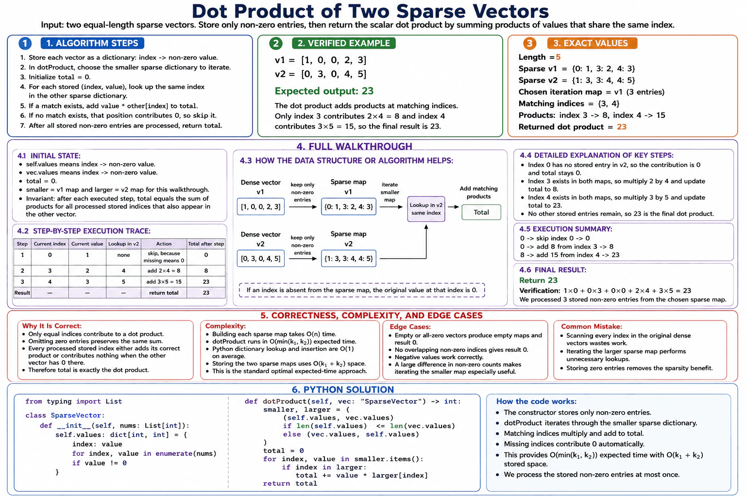
I would store each vector as a dictionary from index to non-zero value. For the dot product, I iterate through the smaller dictionary and look up the same index in the other one. When both vectors contain that index, I multiply the values and add the product to the total. This avoids work on zero entries. Building the sparse maps takes O(n) time. The dot product takes O(min(k1, k2)) expected time, and storage is O(k1 + k2).

The problem asks us to store two vectors efficiently when most values are zero and then calculate their dot product. A dense scan checks every position, including many positions that contribute nothing. Instead, we store only non-zero values in dictionaries. Each dictionary maps an index to the value at that index. We then iterate through the smaller dictionary and check matching indices in the other one.

1. What input sizes, value ranges, and edge cases should the solution handle?
2. What output should be returned for empty, invalid, or duplicate input?
3. Should I prioritize execution time or memory use, and may I use the standard library?

The input is two vectors of the same length. The output is one number: their dot product.

For the example:

v1 = [1, 0, 0, 2, 3]

v2 = [0, 3, 0, 4, 5]

The expected output is 23.

A dot product multiplies values at equal indices and adds the products:

1 × 0 + 0 × 3 + 0 × 0 + 2 × 4 + 3 × 5 = 23.

For each vector, I build a dictionary that maps an index to its non-zero value.

The first vector becomes:

{0: 1, 3: 2, 4: 3}

The second vector becomes:

{1: 3, 3: 4, 4: 5}

If an index is missing from a dictionary, the original value at that position is zero.

I compare the number of stored entries in both dictionaries. I iterate through the smaller dictionary. This reduces the number of lookups when one vector contains fewer non-zero values.

In this example, both dictionaries contain three entries. The walkthrough iterates through the first vector's dictionary.

The invariant is: after each executed step, total equals the sum of the products for all processed stored indices that also appear in the other vector.

Start with total = 0.

At index 0, the first vector stores the value 1. The second dictionary has no entry at index 0. Its original value there is zero, so this position contributes 0. We skip it, and total stays 0.

At index 3, the first vector stores 2. The second vector stores 4 at the same index. We calculate 2 × 4 = 8 and update total from 0 to 8.

At index 4, the first vector stores 3. The second vector stores 5 at the same index. We calculate 3 × 5 = 15 and update total from 8 to 23.

No stored entries remain in the chosen dictionary, so we return 23.

Only values at equal indices contribute to a dot product. Removing zero entries does not change the sum because every product containing zero contributes nothing.

For each stored index in the smaller dictionary, the algorithm checks the same index in the other dictionary. If the index exists, it adds the exact product. If the index is missing, the other value is zero and nothing is added.

Therefore, the final total is exactly the dot product.

The constructor uses enumerate to read each index and value. It stores an entry only when the value is not zero.

The dotProduct method compares the two dictionary sizes and assigns them to smaller and larger. It initializes total to zero. It then loops through each stored index and value in smaller.

When the same index exists in larger, it multiplies the two values and adds the result to total. After all stored entries in smaller have been processed, the method returns total.

Building both sparse representations takes O(n) time overall when each equal-length vector has length n. Each original position is examined once per vector.

The dot product takes O(min(k1, k2)) expected time, where k1 and k2 are the numbers of non-zero entries. Python dictionary lookup is O(1) on average.

The two dictionaries store k1 + k2 entries, so their space use is O(k1 + k2).

Relevant edge cases include all-zero vectors, vectors with no overlapping non-zero indices, negative values, and vectors with very different non-zero counts.

The key insight is that zero values never change a dot-product sum, so they do not need to be stored. Each sparse vector uses a dictionary with index as the key and the non-zero value as the value. The dot product iterates through the smaller dictionary and looks up the same index in the other dictionary. The invariant is that after every processed entry, total equals the sum of the matching products seen so far. This avoids scanning every dense position when most entries are zero.

Let n be the length of each vector. Let k1 and k2 be the numbers of non-zero entries in the two vectors. Building the sparse dictionaries takes O(n) time overall because each vector position is checked once. The dot product takes O(min(k1, k2)) expected time because it loops through the smaller dictionary. A Python dictionary lookup is O(1) on average. The two dictionaries store k1 + k2 entries, so the space use is O(k1 + k2).

A common mistake is scanning every position in the dense vectors, which loses the sparsity benefit. Another mistake is storing zero values in the dictionary and wasting memory. Some candidates iterate through the larger sparse dictionary, which causes unnecessary lookups. Another error is matching equal values instead of matching equal indices. Candidates may also claim guaranteed O(1) dictionary operations, but Python dictionary lookup and insertion are O(1) on average.

First state exactly what the dictionary stores: index maps to non-zero value. Then explain that you iterate through the smaller dictionary and look up the same index in the other one. This makes both the correctness argument and the complexity easy to explain.

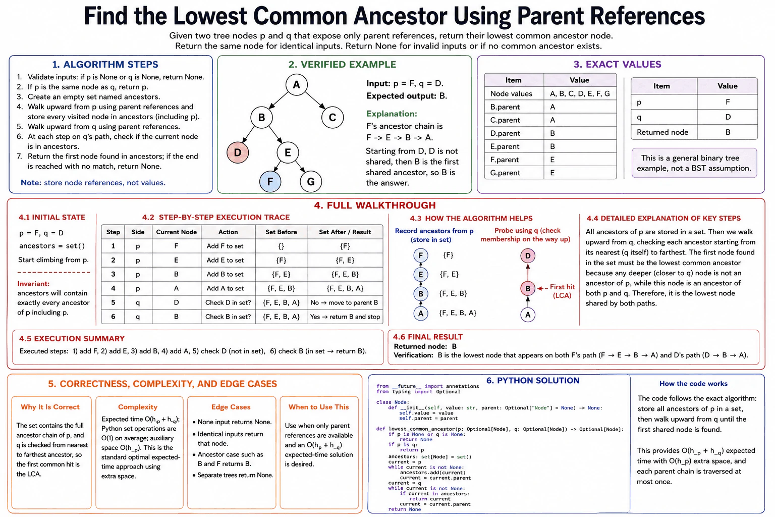
I would store every node on p’s path to the root in a set. Then I would move upward from q and check each node against that set. The first match is the lowest common ancestor because q is checked from its nearest ancestor to its farthest ancestor. For p = F and q = D, the first match is B. The expected time is O(h_p + h_q), and the auxiliary space is O(h_p).

The problem gives two node references, p and q. Each node contains only a parent reference. We must return the lowest node that is an ancestor of both nodes. The diagram uses an ancestor set. First, we record p and every node above p. Then we climb from q and return the first node that appears in that set.

1. What input sizes, value ranges, and edge cases should the solution handle?
2. What output should be returned for empty, invalid, or duplicate input?
3. Should I prioritize execution time or memory use, and may I use the standard library?

The inputs are two node references named p and q. Each node has a value and a parent reference.

The function returns a node reference, not only the node’s value.

If p or q is None, the function returns None. If p and q are the same node object, the function returns that node immediately. If the nodes are in different trees, the second traversal reaches None and the function returns None.

I use a Python set named ancestors.

The set stores node references from p’s path to the root. It does not store only node values because two different nodes could have the same value.

The central invariant is this: after the first traversal, ancestors contains exactly p and every ancestor of p.

I then climb from q. Because I check q’s path from the nearest node to the farthest node, the first node found in ancestors is the lowest common ancestor.

In the diagram, p = F and q = D.

The set starts empty:

ancestors = set()

The first traversal starts at F. At each step, I add the current node to the set and then move to its parent.

The parent relationships are:

B.parent = A C.parent = A D.parent = B E.parent = B F.parent = E G.parent = E

Step 1: The current p-side node is F. The set is empty. Add F. The set becomes {F}. Continue.

Step 2: Move to E. The set is {F}. Add E. The set becomes {F, E}. Continue.

Step 3: Move to B. The set is {F, E}. Add B. The set becomes {F, E, B}. Continue.

Step 4: Move to A. The set is {F, E, B}. Add A. The set becomes {F, E, B, A}. Continue until A.parent is None.

Now begin the second traversal at q = D.

Step 5: Check whether D is in {F, E, B, A}. It is not. Move to D.parent, which is B. Continue.

Step 6: Check whether B is in {F, E, B, A}. It is. Return B and stop immediately.

No node after B is processed because the answer has already been found.

The set contains the complete ancestor chain of F:

F -> E -> B -> A

The upward path from D is:

D -> B -> A

We inspect D’s path from nearest to farthest. D is not shared. B is the first shared node. Therefore, B is the lowest common ancestor.

A higher shared node such as A cannot be the answer because B is below A and is already an ancestor of both F and D.

The function first checks the invalid-input case. It then checks whether p and q are the same object.

Next, it creates an empty set. The first while loop starts at p and adds each node reference before moving to its parent.

The second while loop starts at q. It checks whether the current node is in the set. If it is, the function returns that node immediately. Otherwise, it moves to the parent.

If the second traversal reaches None, the nodes do not share a common ancestor in the same tree, so the function returns None.

Let h_p be the number of nodes from p to the root, including p. Let h_q be the number of nodes from q to the root, including q.

The expected time is O(h_p + h_q). Python set insertion and lookup are O(1) on average.

The auxiliary space is O(h_p) because the set stores p and its ancestors.

Important edge cases are a None input, identical node references, one node already being an ancestor of the other, and nodes that belong to different trees.

The key idea is to save p’s full ancestor chain in a set. Each set entry is a node reference. After the first traversal, the invariant is that the set contains exactly p and every node above p. We then move upward from q in nearest-to-farthest order. The first node found in the set must be the lowest common ancestor. The set is useful because each membership check takes O(1) time on average in Python.

Let h_p be the number of nodes on p’s path to the root, including p. Let h_q be the number of nodes on q’s path to the root, including q. We insert at most h_p node references into the set and check at most h_q node references from q. Python set insertion and lookup are O(1) on average, so the expected time is O(h_p + h_q). The set can hold h_p nodes, so the auxiliary space is O(h_p).

One mistake is storing node values instead of node references. Different nodes can have the same value. Another mistake is forgetting to add p itself to the set. A candidate may also continue climbing after finding B and incorrectly return A. Other common errors are assuming the tree is a binary search tree, forgetting the identical-input case, or describing Python set operations as guaranteed O(1) instead of O(1) on average.

State the invariant before writing code: after the first loop, the set contains exactly p and every ancestor of p. Then explain that checking q from nearest to farthest makes the first set match the lowest common ancestor.

I would first combine all workshop records into a dictionary that maps each year to its total number of classes. Then I examine only years whose previous year is missing, because each of those years starts one consecutive run. From each start, I move forward year by year, add the class counts, and keep the largest total. Each active year is included in one run expansion. The expected time is O(n), and the auxiliary space is O(u) for u unique years.

The problem gives workshop records as pairs of year and class count. We need the largest sum across a consecutive run of active years. A dictionary is a good fit because it combines records for the same year and lets us quickly check whether the previous or next year exists.

1. What input sizes, value ranges, and edge cases should the solution handle?
2. What output should be returned for empty, invalid, or duplicate input?
3. Should I prioritize execution time or memory use, and may I use the standard library?

The input is a list of pairs. Each pair contains a year and a number of classes.

For the example:

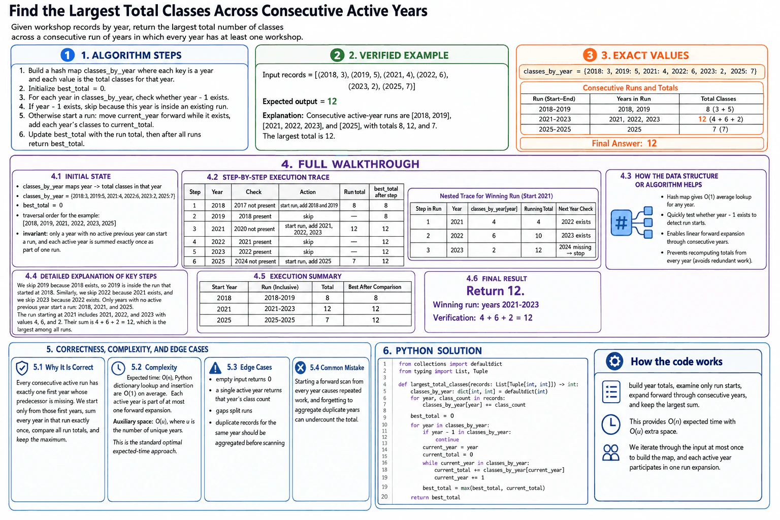
records = [(2018, 3), (2019, 5), (2021, 4), (2022, 6), (2023, 2), (2025, 7)]

The output is one number. It is the largest total classes across any consecutive run of active years.

The active runs are:

2018 to 2019: 3 + 5 = 8

2021 to 2023: 4 + 6 + 2 = 12

2025 to 2025: 7

The required result is 12.

I create a dictionary named classes_by_year.

Each key is a year.

Each value is the total number of classes for that year.

If the same year appears more than once, I add those counts together.

For the example, the dictionary becomes:

{2018: 3, 2019: 5, 2021: 4, 2022: 6, 2023: 2, 2025: 7}

I also initialize best_total to 0.

For each year, I check whether year - 1 exists in the dictionary.

If the previous year exists, the current year is already inside a run. I skip it.

For example, 2019 is skipped because 2018 exists.

The same rule skips 2022 because 2021 exists and skips 2023 because 2022 exists.

A year starts a new run only when its previous year is missing.

When I find a run start, I set current_year to that year and current_total to 0.

Then I move forward while current_year exists in the dictionary.

For the run starting at 2021:

At 2021, I add 4. The running total becomes 4.

At 2022, I add 6. The running total becomes 10.

At 2023, I add 2. The running total becomes 12.

The year 2024 is missing, so the run stops.

I compare 12 with best_total and keep the larger value.

The year 2018 has no active predecessor because 2017 is missing. It starts a run containing 2018 and 2019. The total is 8, so best_total becomes 8.

The year 2019 is skipped because 2018 exists.

The year 2021 has no active predecessor because 2020 is missing. It starts a run containing 2021, 2022, and 2023. The total is 12, so best_total becomes 12.

The years 2022 and 2023 are skipped because each has an active predecessor.

The year 2025 starts a run because 2024 is missing. Its run total is 7, so best_total stays 12.

The function returns 12.

Every consecutive active run has exactly one first year. That first year is the only year in the run whose previous year is missing.

The algorithm starts only from those first years. It then adds every year in that run exactly once.

Because it calculates every run total and keeps the largest one, the final answer is correct.

The first loop builds the year-to-total dictionary.

The second loop checks each unique year. It skips years that are not run starts.

The while loop expands one full consecutive run.

Python dictionary lookup and insertion are O(1) on average.

The expected time is O(n), where n is the number of input records. The auxiliary space is O(u), where u is the number of unique years.

The key insight is that every consecutive active run has exactly one start year. A start year is an active year whose previous year is not present. The dictionary stores year -> total classes for that year. This gives average O(1) checks for whether the previous or next year exists. The central invariant is that only a year with no active predecessor starts a forward scan. Therefore, every active year is counted exactly once as part of one run, and every run total is considered.

The expected time complexity is O(n), where n is the number of input records. Building the dictionary takes O(n). Python dictionary lookup and insertion are O(1) on average. The forward scans take O(u) total because each of the u unique active years belongs to one run expansion. Since u cannot be larger than n, the total expected time is O(n). The auxiliary space is O(u) for the dictionary.

A common mistake is starting a forward scan from every year. That repeats work for years inside the same run. Another mistake is forgetting to combine duplicate records for the same year. Some candidates skip the predecessor check and count the same run more than once. Another error is resetting best_total instead of keeping the maximum. Candidates may also claim guaranteed O(n) time even though Python dictionary operations are O(1) only on average.

State the invariant before writing code: only a year whose previous year is missing can start a run. This makes the skip condition, correctness proof, and expected O(n) analysis easy to explain.

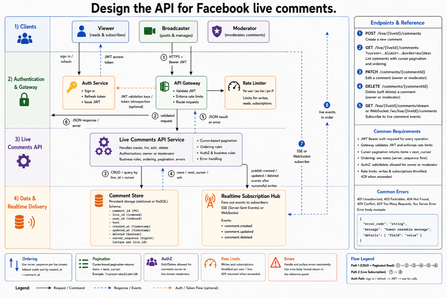
At a high level, I would separate normal comment operations from realtime delivery. Clients sign in through the Auth Service, receive a JWT, and send HTTPS requests through the API Gateway. The gateway validates the JWT, enforces rate limits, and routes requests to the Live Comments API Service. That service creates, lists, edits, or soft-deletes comments in the Comment Store. After a successful write, it publishes an event to the Realtime Subscription Hub. Clients receive ordered events through SSE or WebSocket. This adds operational complexity, but it gives clear security, stable ordering, pagination, and scalable live delivery.

The API must support durable comment operations and immediate live updates. The difficult parts are authorization, stable ordering, pagination, rate control, and consistent error handling. I would explain the design by following the numbered request, response, storage, and subscription flows in the diagram.

1. Which clients and core use cases must the API support?
2. What authentication, authorization, and data-validation rules should I assume?
3. What scale, error handling, idempotency, and versioning requirements matter?

I would start by separating login from normal comment requests. A viewer, broadcaster, or moderator signs in or refreshes a session through the Auth Service. The Auth Service issues a JWT, which is a signed token that identifies the caller.

The client then includes that JWT as a Bearer token on every comment operation. The request uses HTTPS, so the traffic is encrypted while moving across the network.

The main request enters the API Gateway using HTTPS plus the Bearer JWT. The gateway validates the JWT and routes the request. It can obtain validation keys or use token introspection from the Auth Service when needed.

The gateway also enforces rate limits. The Rate Limiter tracks callers per user, live stream, or IP address. It limits writes, reads, and subscriptions. When a caller exceeds the allowed rate, the API returns 429 Too Many Requests.

The visible endpoints are:

• POST /live/{liveId}/comments to create a comment.
• GET /live/{liveId}/comments?cursor=...&limit=...&order=asc|desc to list comments.
• PATCH /comments/{commentId} to edit a comment.
• DELETE /comments/{commentId} to soft-delete a comment.
• GET /live/{liveId}/comments/stream for an SSE subscription.
• WebSocket /ws/live/{liveId}/comments for a live connection.

The gateway forwards the validated request to the Live Comments API Service. This service owns the business rules, authorization, ordering, pagination, and error handling.

Authentication proves who the caller is. Authorization decides what that caller may do. A comment owner may edit or delete their own comment. A moderator may edit or delete any comment allowed by the moderation rules.

The service handles common failures consistently. 401 means authentication is missing or invalid. 403 means the user is authenticated but not allowed. 404 means the requested resource was not found. 409 means the request conflicts with the current state. A limit breach returns 429, while unexpected server failures return a 5xx response.

Errors use a JSON body with error_code, message, and details.

The service reads and writes comment rows in the Comment Store. Each row contains comment_id, live_id, user_id, text, created_at, updated_at, deleted, and server_sequence.

A delete is a soft delete. The row remains stored, but the deleted field marks it as removed.

The server_sequence value is unique within one live stream. It provides stable ordering. The design can use created_at plus comment_id as a fallback stable sort.

The list endpoint uses cursor-based pagination. A cursor identifies the next position in the ordered result. The service returns comment rows plus next_cursor. This works better than page numbers when new comments arrive continuously.

After the service completes the operation, it returns rows, next_cursor, an acknowledgment, or an error to the API Gateway. The gateway then sends the JSON response back to the client.

This is the synchronous path. The request travels from the client to the gateway and service. The response returns from the service through the gateway to the client.

After a successful create, update, or delete, the Live Comments API Service publishes an event to the Realtime Subscription Hub. The supported event names are comment.created, comment.updated, and comment.deleted.

A client opens an SSE or WebSocket subscription for one live stream. The subscription hub manages those connections and fans out events to subscribed clients. The events are delivered in the order defined by the comment sequence.

The normal JSON response and the realtime event are separate flows. The client receives the operation result through the gateway. Other subscribed clients receive the change through the hub.

The benefit is clear responsibility. The gateway handles token checks and rate control. The comments service owns business rules. The store owns durable data. The hub owns realtime fan-out.

The downside is more services and more operational work. We accept this because a busy live stream needs stable ordering, controlled writes, efficient pagination, and many long-lived subscriptions.

The design separates work so each part has one clear job. The gateway checks JWTs, applies rate limits, and routes requests. The comments service handles validation, authorization, ordering, and pagination. The store keeps durable rows. The subscription hub sends live events. Cursor pagination stays stable when new comments arrive, while page numbers may shift. A per-stream sequence gives reliable order, but the service must assign that value carefully. SSE is simple for server-to-client updates. WebSocket supports a longer two-way connection, but it needs more connection management. Soft delete keeps history, but stored data continues growing. The benefit is safer scaling and clearer ownership. The downside is more components, monitoring, and failure points. We accept that cost because live comments create both heavy write traffic and many realtime connections.

At a high level, I would place a versioned REST gateway before four resource APIs: posts, follows, profiles, and feeds. The client first gets a JWT from the Auth Service. It then sends HTTPS requests with that token to the gateway. The gateway validates the token, enforces authorization, applies rate limits, adds a request ID, and routes the call. Each API uses the required data store. Feed requests read follow relationships and recent posts. Cursor pagination keeps changing feeds stable. The trade-off is extra service coordination for clearer ownership and safer request handling.

The goal is to support posting, following, profiles, and feeds through clear APIs. The main challenge is protecting each request while keeping the resource boundaries simple. I would explain the design by following the exact request and response paths in the diagram.

1. Which clients and core use cases must the API support?
2. What authentication, authorization, and data-validation rules should I assume?
3. What scale, error handling, idempotency, and versioning requirements matter?

I would begin with the mobile or web client. The client sends OAuth login credentials to the Auth Service. The Auth Service checks the login and returns an access token as a JWT.

A JWT is a signed token that identifies the caller. The client places it in the Authorization: Bearer JWT header. It then sends the API request over HTTPS.

The request enters the Instagram API Platform through the REST API Gateway and Router. The gateway is the main boundary for the resource APIs.

The gateway accepts HTTPS requests containing JSON. All routes use the /v1 prefix for API versioning.

The gateway validates the Bearer JWT before routing the request. It also enforces authorization before routing. Authentication checks who the caller is. Authorization checks whether that caller may perform the requested action.

The gateway applies rate limiting to control excessive traffic. It also adds a request_id for tracing failures. After these checks, it routes the request to the correct resource API.

To create a post, the gateway sends POST /v1/posts to the Posts API. The request body contains caption and media_url.

The Posts API writes the post to the Posts Store. The store returns the stored post record to the service. The Posts API then returns 201 Created with {post_id, created_at}.

That response moves back to the gateway. The gateway returns the final JSON response to the client.

To follow a user, the gateway sends POST /v1/users/{id}/follow to the Follow API. To unfollow that user, it sends DELETE /v1/users/{id}/follow.

The Follow API creates or removes a follow edge in the Follow Graph Store. A follow edge represents one user following another user. The store returns the resulting follow state.

The Follow API returns either 200 OK or 204 No Content. The response returns through the gateway to the client.

For a profile request, the gateway sends GET /v1/profiles/{username} to the Profile API. The Profile API reads the profile from the Profiles Store. The store returns the profile data. The API then returns 200 OK with profile JSON.

For a feed request, the gateway sends GET /v1/feed?limit=20&cursor=abc123 to the Feed API. The Feed API reads followed accounts from the Follow Graph Store. That store returns the following list.

The Feed API then reads recent posts from the Posts Store. The store returns the post items. The Feed API combines the results and returns {items[], next_cursor} with 200 OK.

The cursor marks where the next page begins. Cursor-based pagination is preferred over offset pagination because feeds change often. It produces more stable pages when new posts arrive.

Validation, authentication, authorization, rate-limit, and service failures are mapped through the error-handling path. The response uses {code, message, details, request_id}.

The diagram shows these common codes. 400 means invalid input. 401 means authentication is missing or invalid. 403 means the caller is authenticated but not allowed. 404 means a resource was not found. 409 means a state conflict. 429 means the rate limit was exceeded. 500 means an unexpected server error.

The benefit of this design is clear ownership and consistent protection. The downside is extra routing and coordination between services. We accept that cost because the boundaries make the system easier to secure, maintain, and extend.

The benefit of separate Posts, Follow, Profile, and Feed APIs is clear ownership. Each API handles one main resource and uses the stores shown in the design. The gateway gives one place for JWT validation, authorization, rate limiting, request IDs, routing, and /v1 versioning. This reduces repeated work inside every API. The downside is that the Feed API needs data from two stores. It reads followed accounts first, then recent posts. That can increase response time. Cursor pagination works well for changing feeds because new posts do not shift every page. Its downside is that cursors are less simple than page numbers. Standard JSON errors help clients handle failures consistently. We accept the extra service coordination because it improves security, ownership, and long-term maintenance.