Microsoft Python Developer Interview Questions & Answers

microsoft icon

Questions with Detailed ExplanationsWith Detailed Explanations

(Last Updated: August 28, 2026)

11. Implement FCFS, SJF, and Round Robin CPU schedulers in Python.Language SpecificHardMicrosoft

Question Details

Implement First-Come, First-Served, Shortest Job First, and Round Robin scheduling. Define the process inputs and output metrics, handle arrival and burst times, and apply the Round Robin quantum correctly.

Short Interview Answer (30-60 seconds)

I would use one validated process model and return the same metrics from all three schedulers. FCFS runs jobs by arrival order. Nonpreemptive SJF chooses the shortest burst among jobs that have arrived. Round Robin uses a deque and runs each ready job for at most one positive quantum. The key detail is to move the clock across idle periods and add arrivals from a completed slice before requeuing unfinished work.

Detailed Explanation

See the Code while reading this explanation.

Use one process model with a unique id, an arrival time, and a positive burst time. Return start, completion, turnaround, waiting, and response time for every process. FCFS sorts by arrival and uses original input order when arrivals are equal. It runs each process to completion. SJF here is nonpreemptive. At each decision point, it selects the arrived process with the smallest burst. If no process is ready, the clock jumps to the next arrival. Round Robin keeps ready processes in collections.deque. It runs the front process for the smaller of its remaining burst and the positive quantum. Arrivals that occur during that slice enter the queue before the unfinished process is added back. Turnaround is completion minus arrival. Waiting is turnaround minus burst. Response is first start minus arrival. FCFS is simple but short work may wait behind long work. SJF can reduce average waiting when burst estimates are useful, but long work may wait too long. Round Robin improves fairness and response, but a small quantum causes more queue turns and real context switches. This code is a deterministic simulator. A production operating system also handles priorities, interrupts, context switch cost, and changing workloads.

Useful Questions to Ask the Interviewer
  1. Should I focus on Python language behavior, or also explain the runtime and standard library?
  2. Which Python version and execution environment should I assume?
  3. Would you like a small code example together with production tradeoffs and edge cases?
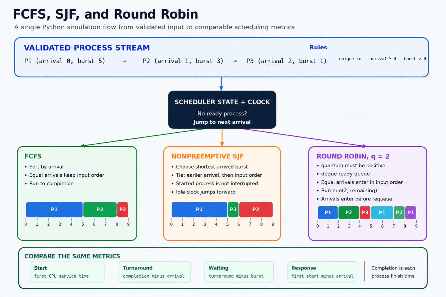
Implement FCFS, SJF, and Round Robin CPU schedulers in Python. diagram
Example

The code validates every process and returns results in original input order. FCFS uses one stable sort and takes O(n log n) time. The shown SJF scans pending work for every selection and takes O(n squared) time. Round Robin sorts arrivals once and performs one constant time queue turn per slice. Its time is O(n log n plus k), where k is the total number of slices, equal to the sum of ceiling of burst divided by quantum for all processes. Every scheduler uses O(n) extra memory. For P1 with arrival 0 and burst 5, P2 with arrival 1 and burst 3, and P3 with arrival 2 and burst 1, FCFS gives completion times 5, 8, and 9. Nonpreemptive SJF gives 5, 9, and 6. Round Robin with quantum 2 gives 9, 8, and 5. All three use the same turnaround, waiting, and response formulas.

Code
from collections import deque
from dataclasses import dataclass
from typing import Callable


@dataclass(frozen=True)
class Process:
    pid: str
    arrival: int
    burst: int


MetricRow = dict[str, int | str]


def validate(processes: list[Process]) -> None:
    # Every process needs a unique id, a nonnegative arrival, and positive work.
    if len({process.pid for process in processes}) != len(processes):
        raise ValueError("Process ids must be unique")

    for process in processes:
        if process.arrival < 0:
            raise ValueError("Arrival time cannot be negative")
        if process.burst <= 0:
            raise ValueError("Burst time must be positive")


def make_result(
    process: Process,
    start: int,
    completion: int,
) -> MetricRow:
    # Turnaround is the total time from arrival through completion.
    turnaround = completion - process.arrival
    # Waiting excludes the time spent using the CPU.
    waiting = turnaround - process.burst
    # Response is the delay before the first CPU service.
    response = start - process.arrival

    return {
        "pid": process.pid,
        "arrival": process.arrival,
        "burst": process.burst,
        "start": start,
        "completion": completion,
        "turnaround": turnaround,
        "waiting": waiting,
        "response": response,
    }


def fcfs(processes: list[Process]) -> list[MetricRow]:
    validate(processes)

    # Python sorting is stable. The index makes the equal arrival rule explicit.
    ordered = sorted(
        enumerate(processes),
        key=lambda item: (item[1].arrival, item[0]),
    )
    time = 0
    by_index: dict[int, MetricRow] = {}

    for index, process in ordered:
        # Jump over an idle period when the next process has not arrived.
        start = max(time, process.arrival)
        completion = start + process.burst
        by_index[index] = make_result(process, start, completion)
        time = completion

    # Return every scheduler result in original input order.
    return [by_index[index] for index in range(len(processes))]


def sjf(processes: list[Process]) -> list[MetricRow]:
    validate(processes)

    # This is nonpreemptive SJF. A started process runs to completion.
    pending = list(enumerate(processes))
    time = 0
    by_index: dict[int, MetricRow] = {}

    while pending:
        ready = [item for item in pending if item[1].arrival <= time]

        if not ready:
            # No process is ready, so move directly to the next arrival.
            time = min(process.arrival for _, process in pending)
            ready = [item for item in pending if item[1].arrival <= time]

        index, process = min(
            ready,
            key=lambda item: (
                item[1].burst,
                item[1].arrival,
                item[0],
            ),
        )

        start = time
        completion = start + process.burst
        by_index[index] = make_result(process, start, completion)
        time = completion
        pending.remove((index, process))

    return [by_index[index] for index in range(len(processes))]


def round_robin(
    processes: list[Process],
    quantum: int,
) -> list[MetricRow]:
    validate(processes)

    if quantum <= 0:
        raise ValueError("Quantum must be positive")

    ordered = sorted(
        enumerate(processes),
        key=lambda item: (item[1].arrival, item[0]),
    )
    remaining = {index: process.burst for index, process in ordered}
    first_start: dict[int, int] = {}
    completion: dict[int, int] = {}
    ready: deque[int] = deque()
    time = 0
    next_arrival = 0

    while next_arrival < len(ordered) or ready:
        if not ready:
            # Jump over an idle period.
            time = max(time, ordered[next_arrival][1].arrival)

            # Add every process that is available at the new time.
            while next_arrival < len(ordered) and ordered[next_arrival][1].arrival <= time:
                ready.append(next_arrival)
                next_arrival += 1

        # The queue stores positions inside the arrival ordered list.
        position = ready.popleft()
        original_index, process = ordered[position]
        first_start.setdefault(original_index, time)

        run_time = min(quantum, remaining[original_index])
        time += run_time
        remaining[original_index] -= run_time

        # Add arrivals from this slice before requeuing unfinished work.
        while next_arrival < len(ordered) and ordered[next_arrival][1].arrival <= time:
            ready.append(next_arrival)
            next_arrival += 1

        if remaining[original_index] > 0:
            ready.append(position)
        else:
            completion[original_index] = time

    return [
        make_result(
            process,
            first_start[index],
            completion[index],
        )
        for index, process in enumerate(processes)
    ]


def print_schedule(
    name: str,
    scheduler: Callable[[], list[MetricRow]],
) -> None:
    print(f"\n{name}")
    for row in scheduler():
        print(row)


if __name__ == "__main__":
    sample = [
        Process("P1", arrival=0, burst=5),
        Process("P2", arrival=1, burst=3),
        Process("P3", arrival=2, burst=1),
    ]

    print_schedule("FCFS", lambda: fcfs(sample))
    print_schedule("SJF", lambda: sjf(sample))
    print_schedule(
        "Round Robin with quantum 2",
        lambda: round_robin(sample, quantum=2),
    )
Where it is used

These schedulers are useful in operating system teaching tools, workload simulators, interview exercises, and tests for queue based dispatch logic. Similar ideas appear in worker pools, job runners, request queues, and time sharing services. Real production schedulers usually add priorities, cancellation, resource limits, context switch cost, and dynamic workload information.

Why Interviewers Ask This

Interviewers ask this question to test whether a candidate can turn scheduling rules into correct Python state changes. It checks stable sorting, queue operations with collections.deque, clock movement, validation, tie handling, and metric calculation. It also tests whether the candidate understands arrivals, remaining work, fairness, idle periods, and the effect of the Round Robin quantum.

Common interview mistakes

Common mistakes include choosing an SJF process before checking its arrival, treating SJF as preemptive without saying so, ignoring idle CPU periods, allowing a zero or negative quantum, and resetting burst time instead of tracking remaining work. Other errors include calculating response from the last start, requeuing the current Round Robin process before adding arrivals from its completed slice, using completion minus burst as waiting when arrival is not zero, and leaving equal arrival ties undefined.

Interview tip

State the assumptions first. Say that SJF is nonpreemptive, equal ties use original input order, and the quantum must be positive. Then explain the ready set, clock movement, and the metric formulas. Walk through one Round Robin slice and state exactly when new arrivals enter the deque.
Interviewer may ask next
What happens when no process is ready at the current time?

The scheduler moves the clock directly to the next arrival time. This exact clock jump represents an idle CPU period and prevents the simulation from getting stuck. FCFS handles it with the larger of the current clock and the next arrival. SJF and Round Robin perform the jump before selecting or dequeuing work.

How does the Round Robin quantum affect performance and fairness?

A smaller quantum gives ready processes more frequent turns and can improve response time, but it increases the number of slices and real context switches. A larger quantum reduces that overhead, but response can become slower and the behavior approaches FCFS. The production tradeoff depends on workload lengths, latency goals, and context switch cost.

12. Design a Python logging framework for multiple modules with concurrent writers.Language SpecificHardMicrosoft

Question Details

Several controller or module threads write log records to a shared buffer, while a framework thread streams them to a file or external tool and acknowledges records only after they are written. Define the interfaces, synchronization, buffering, ordering, backpressure, shutdown, and failure behavior.

Short Interview Answer (30-60 seconds)

I would give every module one submit interface backed by a bounded Queue and use one framework thread as the only destination writer. Queue safely coordinates Python threads, while the single writer preserves queue insertion order and prevents overlapping writes. A receipt is completed only after write and flush succeed. Producers wait or receive a timeout error when the queue is full. Shutdown rejects new submissions, places a stop marker after accepted records, drains them, joins the writer, and then closes the destination.

Detailed Explanation

See the Code while reading this explanation.

I would use a bounded Queue from the Python standard library and one dedicated writer thread. Each module submits a copied LogRecord and receives a LogReceipt. Queue provides locking and waiting behavior, so producers do not share a list directly. The writer alone touches the file or external tool adapter.

Useful Questions to Ask the Interviewer
  1. Should I focus on Python language behavior, or also explain the runtime and standard library?
  2. Which Python version and execution environment should I assume?
  3. Would you like a small code example together with production tradeoffs and edge cases?

Records are processed in queue insertion order. Threads that create records at nearly the same time have no stronger global order. Each receipt contains an Event. The writer completes it only after write and flush succeed. Flush does not always mean durable disk storage or remote acceptance, so a stricter sink must call fsync or wait for the external tool response.

The queue has a fixed capacity. This bounds queued memory and creates backpressure. A producer may wait, use a timeout, or reject lower priority logs.

Shutdown first blocks new submissions. It then places a stop marker after every accepted item and joins the writer. A destination error fails the current receipt, marks the logger failed, rejects later submissions, and fails remaining queued receipts. Queue operations are constant time in normal use. Serialization and writing cost depend on record size, and queued memory grows with capacity and record size.

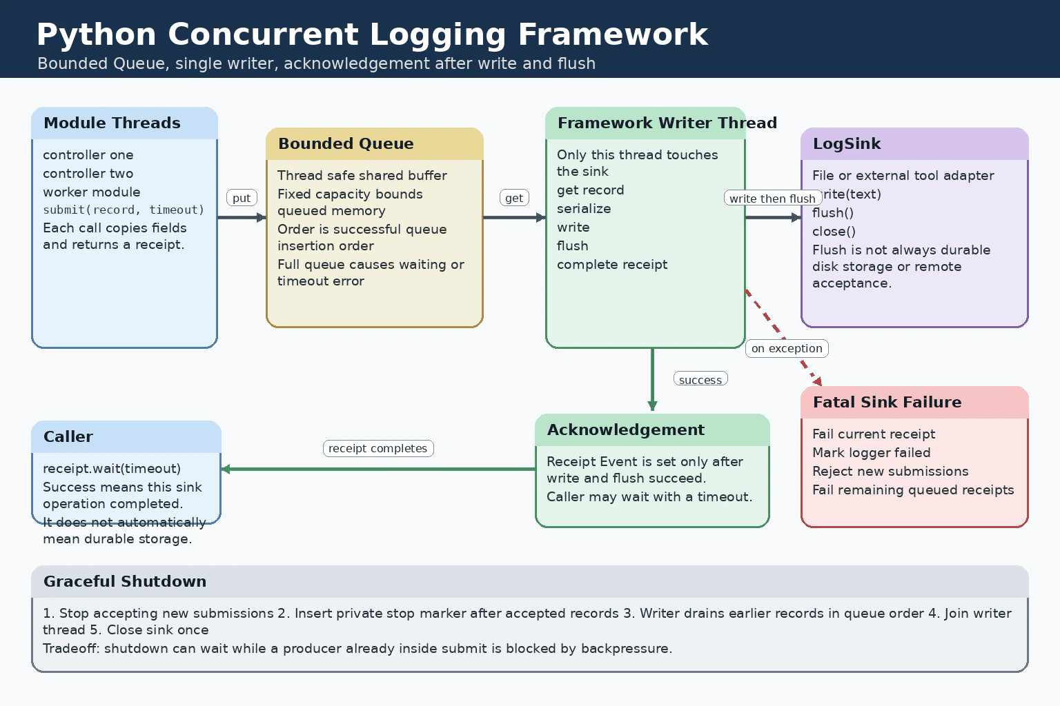
Design a Python logging framework for multiple modules with concurrent writers. diagram
Example

The implementation defines a LogSink interface for a file or external adapter. A bounded Queue is the shared buffer. Queue.put and Queue.get provide thread synchronization. submit deep copies the fields so later caller changes, including nested changes, cannot alter an accepted record. The copied mapping is exposed as read only. Each submission returns a LogReceipt with an Event. The writer completes the receipt only after sink write and flush succeed. One writer thread owns the sink, so destination calls never overlap. The state lock makes submission and shutdown share one clear acceptance boundary. When the queue remains full past the chosen timeout, submit raises LoggingBackpressureError. Shutdown rejects new records, inserts a private stop marker after accepted records, joins the writer, and closes the sink once. A sink failure marks the framework failed. The current receipt and later queued receipts receive that failure, and new submissions are rejected.

Code
from __future__ import annotations

import copy
import io
import json
import queue
import threading
import time
from dataclasses import dataclass, field
from types import MappingProxyType
from typing import Any, Mapping, Protocol


class LogSink(Protocol):
    # A file or external tool adapter must provide these operations.
    def write(self, text: str) -> int: ...

    def flush(self) -> None: ...

    def close(self) -> None: ...


class LoggingFrameworkError(Exception):
    # Base exception for framework failures.
    pass


class LoggingClosedError(LoggingFrameworkError):
    # Raised when submission happens after shutdown starts.
    pass


class LoggingBackpressureError(LoggingFrameworkError):
    # Raised when the bounded queue stays full past the timeout.
    pass


@dataclass(frozen=True)
class LogRecord:
    # The record data is isolated from later caller changes.
    timestamp: float
    module: str
    level: str
    message: str
    fields: Mapping[str, Any] = field(default_factory=dict)


class LogReceipt:
    # A caller may wait until the writer finishes this record.
    def __init__(self) -> None:
        self._done = threading.Event()
        self._error: Exception | None = None

    def _complete(self, error: Exception | None = None) -> None:
        self._error = error
        self._done.set()

    def wait(self, timeout: float | None = None) -> None:
        # Return only after success or a confirmed delivery failure.
        if not self._done.wait(timeout):
            raise TimeoutError("Log acknowledgement timed out")
        if self._error is not None:
            raise LoggingFrameworkError("Log delivery failed") from self._error


@dataclass
class _QueuedRecord:
    record: LogRecord
    receipt: LogReceipt


_STOP = object()


class ConcurrentLogger:
    def __init__(self, sink: LogSink, capacity: int = 1000) -> None:
        if capacity <= 0:
            raise ValueError("capacity must be positive")

        self._sink = sink
        self._queue: queue.Queue[_QueuedRecord | object] = queue.Queue(maxsize=capacity)
        self._state_lock = threading.Lock()
        self._shutdown_lock = threading.Lock()
        self._failure_lock = threading.Lock()
        self._accepting = True
        self._fatal_error: Exception | None = None
        self._failed = threading.Event()

        self._writer = threading.Thread(
            target=self._writer_loop,
            name="logging framework writer",
            daemon=False,
        )
        self._writer.start()

    def submit(
        self,
        module: str,
        level: str,
        message: str,
        fields: Mapping[str, Any] | None = None,
        timeout: float | None = None,
    ) -> LogReceipt:
        # Deep copy the fields so nested caller data cannot change later.
        safe_fields = copy.deepcopy(dict(fields or {}))
        record = LogRecord(
            timestamp=time.time(),
            module=module,
            level=level,
            message=message,
            fields=MappingProxyType(safe_fields),
        )
        receipt = LogReceipt()
        item = _QueuedRecord(record=record, receipt=receipt)

        # Keep shutdown from placing the stop marker before this put finishes.
        with self._state_lock:
            if not self._accepting:
                raise LoggingClosedError("Logging framework is closing")

            if self._failed.is_set():
                raise LoggingFrameworkError(
                    "Logging framework has failed"
                ) from self._get_fatal_error()

            try:
                self._queue.put(item, block=True, timeout=timeout)
            except queue.Full as error:
                raise LoggingBackpressureError("Logging queue is full") from error

        return receipt

    def shutdown(self) -> None:
        # Serialize shutdown so the sink is closed exactly once.
        with self._shutdown_lock:
            with self._state_lock:
                if self._accepting:
                    self._accepting = False
                    # This marker enters after all accepted records.
                    self._queue.put(_STOP)

            # Wait until the writer processes accepted records and the marker.
            self._writer.join()

            try:
                self._sink.close()
            except Exception as error:
                self._set_fatal_error(error)

            error = self._get_fatal_error()
            if error is not None:
                raise LoggingFrameworkError("Logging framework stopped after a failure") from error

    def _set_fatal_error(self, error: Exception) -> None:
        with self._failure_lock:
            if self._fatal_error is None:
                self._fatal_error = error
                self._failed.set()

    def _get_fatal_error(self) -> Exception | None:
        with self._failure_lock:
            return self._fatal_error

    def _writer_loop(self) -> None:
        while True:
            item = self._queue.get()
            try:
                if item is _STOP:
                    return

                assert isinstance(item, _QueuedRecord)

                existing_error = self._get_fatal_error()
                if existing_error is not None:
                    item.receipt._complete(existing_error)
                    continue

                try:
                    text = json.dumps(
                        {
                            "timestamp": item.record.timestamp,
                            "module": item.record.module,
                            "level": item.record.level,
                            "message": item.record.message,
                            "fields": dict(item.record.fields),
                        },
                        sort_keys=True,
                    )
                    self._sink.write(text + "\n")
                    self._sink.flush()
                    item.receipt._complete()
                except Exception as error:
                    # One sink failure makes this logger fail closed.
                    self._set_fatal_error(error)
                    item.receipt._complete(error)
            finally:
                self._queue.task_done()


def main() -> None:
    # StringIO makes the example runnable without creating a file.
    output = io.StringIO()
    logger = ConcurrentLogger(output, capacity=10)

    receipts: list[LogReceipt] = []
    receipts_lock = threading.Lock()

    def controller(name: str) -> None:
        for number in range(3):
            receipt = logger.submit(
                module=name,
                level="INFO",
                message="controller update",
                fields={"number": number},
                timeout=1.0,
            )
            with receipts_lock:
                receipts.append(receipt)

    threads = [
        threading.Thread(target=controller, args=("module one",)),
        threading.Thread(target=controller, args=("module two",)),
    ]

    for thread in threads:
        thread.start()
    for thread in threads:
        thread.join()

    # Wait for acknowledgement of every accepted record.
    for receipt in receipts:
        receipt.wait(timeout=2.0)

    # Read the output before shutdown closes StringIO.
    rendered_output = output.getvalue()
    logger.shutdown()
    print(rendered_output, end="")


if __name__ == "__main__":
    main()
Where it is used

This design is used in web services, worker processes, controller software, test frameworks, and desktop applications where many Python modules produce logs but one file, socket, or external tool must receive them in a controlled sequence. It is useful when the process needs bounded buffering, optional delivery confirmation, and a shutdown path that does not silently discard accepted records.

Why Interviewers Ask This

Interviewers ask this question to test whether the candidate understands Python thread coordination, queue behavior, file ownership, failure propagation, and clean shutdown. It also tests practical judgment about ordering, bounded memory, acknowledgement, backpressure, and the boundary between an accepted record and a rejected record.

Common interview mistakes

Common mistakes include letting all producers write directly to the same destination, using an unbounded queue, and treating queue insertion as proof that the destination accepted the record. Other mistakes are acknowledging before flush succeeds, claiming timestamp order across threads, sharing mutable field data without copying it, using a daemon writer that can disappear during process exit, and placing the stop marker before submissions are blocked. It is also wrong to claim that flush guarantees durable disk storage or confirmation from a remote tool.

Interview tip

Explain the design in this order: one writer, bounded queue, receipt after write and flush, queue insertion order, backpressure, shutdown boundary, then failure propagation. State the durability limit of flush so the guarantee is precise.

Interviewer may ask next
What happens if shutdown starts while a producer is submitting a record?

The state lock defines the exact acceptance boundary. A producer that already holds the lock may finish its queue insertion before shutdown changes the accepting state. That record is accepted and appears before the stop marker. A producer that reaches the lock after shutdown changes the state receives LoggingClosedError. This matters because every accepted record is processed before the writer exits. The tradeoff is that shutdown can wait while an accepted producer is blocked by queue backpressure.

How would you provide stronger delivery guarantees than write and flush?

I would keep the same queue, receipt, and single writer design but strengthen the LogSink contract. For a file sink, the writer could flush and then call os.fsync on the file descriptor before completing the receipt. For an external tool, the adapter could wait for a protocol acknowledgement. This matters when loss after an operating system or network buffer is unacceptable. The tradeoff is much higher latency and lower throughput for every acknowledged record.

13. Find the minimum cycle cost for every node.CodingHardMicrosoft

Question Details

Given a weighted directed graph, determine the minimum cycle cost associated with every node and define the result for nodes that do not belong to a qualifying cycle.

Short Interview Answer (30-60 seconds)

I would compute all-pairs shortest paths with Floyd–Warshall. I also store the incoming edges for each node. For a node s and an incoming edge u → s with weight w, the cheapest cycle using that final edge costs dist[s][u] + w. I take the minimum valid candidate. If no incoming edge can close a cycle, I return -1. The total time is O(n³ + m), and the auxiliary space is O(n² + m).

Detailed Explanation

See the Code while reading this explanation.

The input is a weighted directed graph with n nodes and edges written as (u, v, w). We must return the minimum directed-cycle cost for every node. A node that is not part of any directed cycle gets -1. The solution uses Floyd–Warshall because it computes the shortest path between every ordered pair of nodes. Those paths let us close each possible cycle with an incoming edge.

Useful Questions to Ask the Interviewer
  1. What input sizes, value ranges, and edge cases should the solution handle?
  2. What output should be returned for empty, invalid, or duplicate input?
  3. Should I prioritize execution time or memory use, and may I use the standard library?
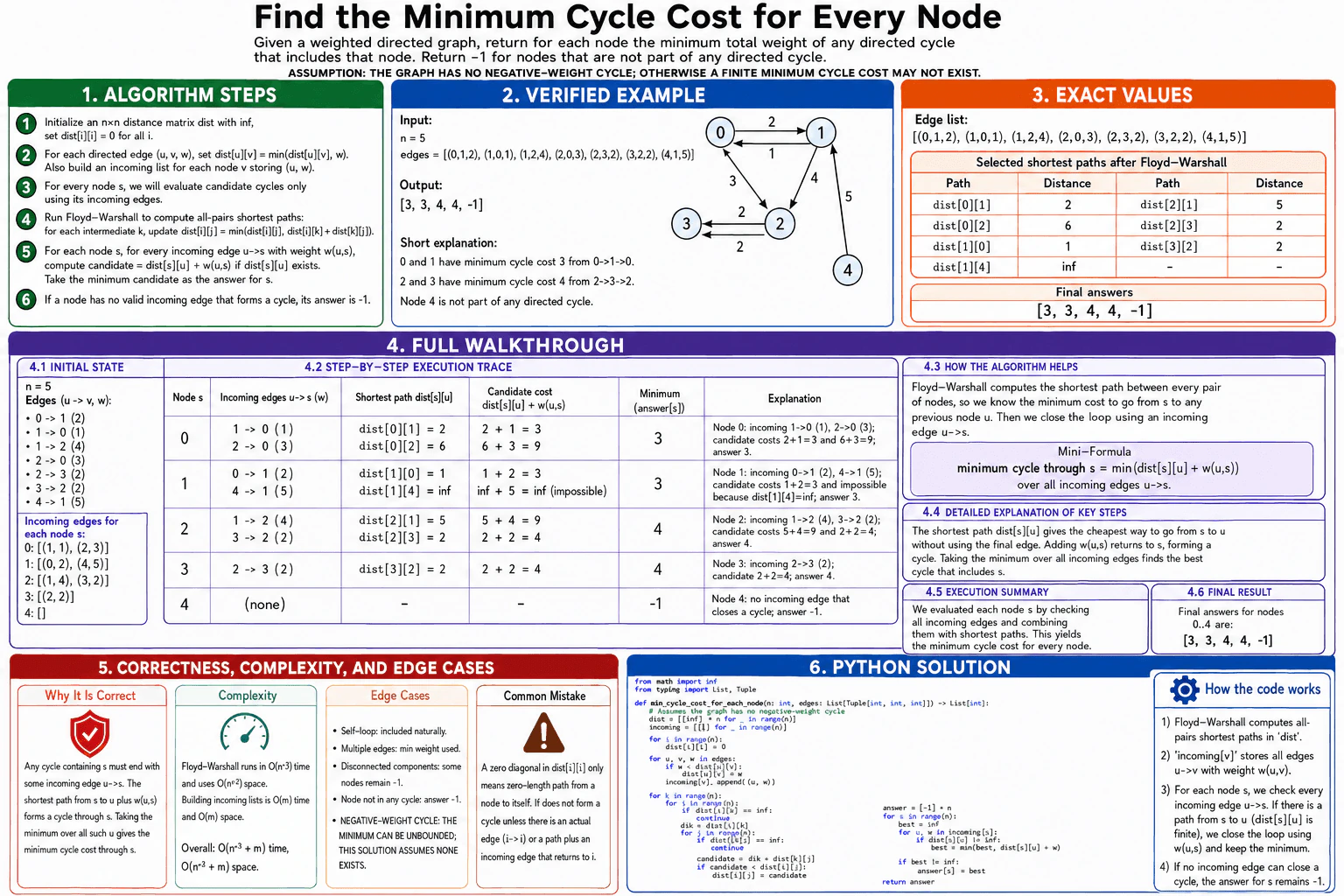
Find the minimum cycle cost for every node. diagram
How to Explain It in an Interview
1. Define the input and required output

Each tuple (u, v, w) represents a directed edge from node u to node v with weight w.

The result is an array of length n. The value at index s is the minimum total weight of a directed cycle that contains node s. If no directed cycle contains s, the result for that node is -1.

The solution assumes the graph has no negative-weight cycle. If a negative-weight cycle exists, its cost can be repeated and the minimum may be unbounded.

2. Initialize the distance matrix and incoming-edge lists

Create an n × n matrix called dist.

Set dist[i][i] to 0. Set every other entry to infinity. For every edge u → v with weight w, set dist[u][v] to the smallest direct weight seen for that ordered pair.

Also create incoming[v]. It stores pairs (u, w) for every edge u → v. This lets us quickly inspect every possible final edge of a cycle through v.

3. Run Floyd–Warshall

For every intermediate node k, try to improve each path i → j by going through k.

The update is:

dist[i][j] = min(dist[i][j], dist[i][k] + dist[k][j])

After all iterations, dist[i][j] is the minimum path cost from i to j. It remains infinity when no path exists.

4. Calculate the minimum cycle cost for each node

Consider a node s. Every directed cycle through s must finish with some incoming edge u → s.

If dist[s][u] is finite, there is a path from s to u. Adding the edge u → s closes a directed cycle through s.

The candidate cost is:

dist[s][u] + w(u, s)

Check every incoming edge and keep the smallest candidate. If no candidate exists, return -1 for that node.

5. Walk through the verified example

The example is:

n = 5

edges = [(0, 1, 2), (1, 0, 1), (1, 2, 4), (2, 0, 3), (2, 3, 2), (3, 2, 2), (4, 1, 5)]

For node 0, the incoming edges are 1 → 0 with weight 1 and 2 → 0 with weight 3. Floyd–Warshall gives dist[0][1] = 2 and dist[0][2] = 6. The candidates are 2 + 1 = 3 and 6 + 3 = 9. The minimum is 3.

For node 1, the incoming edges are 0 → 1 with weight 2 and 4 → 1 with weight 5. We have dist[1][0] = 1, so the first candidate is 1 + 2 = 3. We have dist[1][4] = infinity, so the second edge cannot close a cycle. The answer is 3.

For node 2, the incoming edges are 1 → 2 with weight 4 and 3 → 2 with weight 2. We have dist[2][1] = 5 and dist[2][3] = 2. The candidates are 5 + 4 = 9 and 2 + 2 = 4. The answer is 4.

For node 3, the incoming edge is 2 → 3 with weight 2. Since dist[3][2] = 2, the cycle cost is 2 + 2 = 4.

Node 4 has no incoming edge. No directed cycle can contain it, so its answer is -1.

The final result is [3, 3, 4, 4, -1].

6. Explain why the algorithm is correct

Every directed cycle through s has a final incoming edge u → s. Before using that edge, the cycle contains a path from s to u.

Floyd–Warshall gives the minimum possible cost of that path. Therefore, dist[s][u] + w(u, s) is the cheapest cycle that uses u → s as its final edge.

Taking the minimum over every incoming edge gives the minimum cycle cost through s.

7. Explain the code, complexity, and edge cases

The code builds dist and incoming, runs Floyd–Warshall, and then evaluates every incoming edge for every node.

Floyd–Warshall takes O(n³) time. Building the graph state and checking all incoming edges takes O(m) time. The total time is O(n³ + m).

The distance matrix uses O(n²) space. The incoming-edge lists use O(m) space. The total auxiliary space is O(n² + m).

Important cases include self-loops, parallel edges, disconnected components, and nodes that do not belong to any directed cycle. The solution assumes there is no negative-weight cycle.

Key Insight / Why This Solution Works

The main insight is that every directed cycle through node s must end with an incoming edge u → s. Once all shortest paths are known, the cheapest cycle using that final edge has cost dist[s][u] + w(u, s). Floyd–Warshall is suitable because it computes dist for every ordered pair of nodes. The central invariant is that, after Floyd–Warshall finishes, dist[i][j] stores the minimum path cost from i to j. The minimum valid candidate over all incoming edges gives the answer for s.

Code
from math import inf
from typing import List, Tuple


def min_cycle_cost_for_each_node(
    n: int,
    edges: List[Tuple[int, int, int]],
) -> List[int]:
    """Return the minimum directed-cycle cost for every node.

    A node that is not part of any directed cycle receives -1.
    The graph is assumed to have no negative-weight cycle.
    """

    # Step 1: Initialize the all-pairs distance matrix.
    # dist[i][j] stores the shortest known path cost from i to j.
    dist = [[inf] * n for _ in range(n)]

    for node in range(n):
        dist[node][node] = 0

    # incoming[v] stores every edge u -> v as (u, weight).
    incoming: List[List[Tuple[int, int]]] = [[] for _ in range(n)]

    # Step 2: Store direct edges and build incoming-edge lists.
    for u, v, weight in edges:
        # Keep the cheapest direct edge when parallel edges exist.
        dist[u][v] = min(dist[u][v], weight)
        incoming[v].append((u, weight))

    # Step 3: Compute all-pairs shortest paths with Floyd-Warshall.
    for k in range(n):
        for i in range(n):
            if dist[i][k] == inf:
                continue

            for j in range(n):
                if dist[k][j] == inf:
                    continue

                candidate_distance = dist[i][k] + dist[k][j]
                if candidate_distance < dist[i][j]:
                    dist[i][j] = candidate_distance

    # Step 4: Find the minimum cycle cost for every node.
    answer = [-1] * n

    for s in range(n):
        best_cycle_cost = inf

        # Every cycle through s must end with an incoming edge u -> s.
        for u, weight in incoming[s]:
            if dist[s][u] != inf:
                cycle_cost = dist[s][u] + weight
                best_cycle_cost = min(best_cycle_cost, cycle_cost)

        if best_cycle_cost != inf:
            answer[s] = best_cycle_cost

    return answer


if __name__ == "__main__":
    node_count = 5
    graph_edges = [
        (0, 1, 2),
        (1, 0, 1),
        (1, 2, 4),
        (2, 0, 3),
        (2, 3, 2),
        (3, 2, 2),
        (4, 1, 5),
    ]

    result = min_cycle_cost_for_each_node(node_count, graph_edges)
    print(result)  # [3, 3, 4, 4, -1]
Time & Space Complexity

Let n be the number of nodes and m be the number of directed edges. Floyd–Warshall uses three nested loops, so it takes O(n³) time. Reading the edges and evaluating all incoming edges takes O(m) time. The total time is O(n³ + m). The n × n distance matrix uses O(n²) extra memory. The incoming-edge lists store O(m) entries. Therefore, the auxiliary space complexity is O(n² + m).

Where it is used

This approach is useful when the graph is small or dense and we need shortest-path or cycle information for many different nodes. Similar techniques appear in routing analysis, dependency graphs, transportation networks, workflow loops, and systems that must find the cheapest way to leave a state and return to it.

Why Interviewers Ask This

The interviewer is testing whether you can turn a cycle problem into an all-pairs shortest-path problem. They want to see correct handling of directed edges, a clear distance-state definition, and a valid correctness argument. They also evaluate whether you can connect the mathematical formula to working Python code, handle nodes outside all cycles, discuss parallel edges and disconnected parts, and state the O(n³ + m) time and O(n² + m) space accurately.

Common interview mistakes

A common mistake is returning dist[s][s] = 0 as the cycle cost. That is only the empty path, not a real cycle. Another mistake is checking outgoing edges while using the formula for incoming edges. Candidates may also reverse an edge direction, forget to keep the smallest parallel edge, or add infinity to a weight without first checking reachability. It is also incorrect to claim that the method produces a finite minimum when a negative-weight cycle is present.

Interview tip

State the formula early: for every incoming edge u → s, the candidate cycle cost is dist[s][u] + w(u, s). Then explain why every cycle through s must end with one such edge.

Interviewer may ask next
What changes if the graph can contain a negative-weight cycle?

After Floyd–Warshall, a node k with dist[k][k] < 0 belongs to or can represent a negative-weight cycle. For each node s, we must determine whether s can reach such a cycle and whether the cycle can reach a node u that has an incoming edge u → s. If so, the minimum cycle cost through s is unbounded rather than finite. The time remains O(n³), and the space remains O(n² + m). The output contract must use a separate value for an unbounded result.

Can the O(n²) distance-matrix space be reduced for a sparse graph?

If every edge weight is nonnegative, run Dijkstra once from each node and evaluate that node's incoming edges immediately. This uses about O(n + m) working space per run instead of storing the full distance matrix. The time becomes O(n(m + n) log n) with a binary heap. The tradeoff is more repeated work, and Dijkstra cannot be used when negative edges exist.

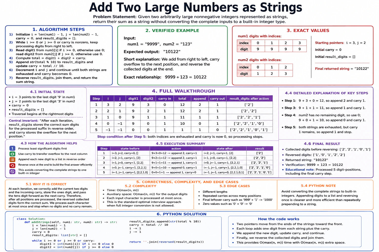
14. Add two large numbers represented as strings.CodingEasyMicrosoft

Question Details

Given two arbitrarily large nonnegative integers represented as strings, return their sum as a string without converting the complete inputs to a built-in integer type.

Short Interview Answer (30-60 seconds)

I add the numbers one digit at a time from right to left, just like manual addition. I keep one pointer for each string and a carry value for overflow. In every loop, I add the current digits and the carry, append the ones digit, and move both pointers left. After both strings and the final carry are processed, I reverse the collected digits and join them. The time complexity is O(max(n, m)), and the auxiliary space complexity is O(max(n, m)).

Detailed Explanation

See the Code while reading this explanation.

The input contains two nonnegative integers stored as strings. We must return their sum as another string without converting either complete input into a built-in integer. The selected method copies manual addition. We process digits from right to left, keep a carry for overflow, and collect the answer digits in reverse order.

Useful Questions to Ask the Interviewer
  1. What input sizes, value ranges, and edge cases should the solution handle?
  2. What output should be returned for empty, invalid, or duplicate input?
  3. Should I prioritize execution time or memory use, and may I use the standard library?
Add two large numbers represented as strings. diagram
How to Explain It in an Interview
1. Understand the input and required output

The inputs are num1 and num2. Each string represents one nonnegative integer. The output must be a string that represents their sum.

For the diagram example, num1 is "9999" and num2 is "123". The required output is "10122" because 9999 + 123 = 10122.

We must not convert either complete string into an integer. We only convert one digit character at a time.

2. Choose right-to-left digit addition

Normal addition starts with the least significant digits. These are the digits on the right side.

Pointer i starts at index 3 in num1, where the digit is 9. Pointer j starts at index 2 in num2, where the digit is 3.

The carry starts at 0. The result_digits list starts empty.

The central invariant is: after each iteration, result_digits stores the correct sum digits for the processed suffix in reverse order, and carry stores the overflow for the next position.

3. Process one digit position at a time

The loop continues while i is valid, j is valid, or carry is nonzero.

If one string has no remaining digit, we use 0 for that string. We calculate total = digit1 + digit2 + carry.

We append str(total % 10). This is the ones digit of the current total. We then set carry = total // 10. This is the overflow for the next position.

Finally, we decrement both pointers so they move one position to the left.

4. Walk through the exact example

Step 1 starts with i = 3, j = 2, and carry = 0. The current digits are 9 and 3. We calculate 9 + 3 + 0 = 12. We append "2" and set carry to 1. result_digits becomes ["2"].

Step 2 uses digits 9 and 2 with carry 1. We calculate 9 + 2 + 1 = 12. We append "2" and keep carry as 1. result_digits becomes ["2", "2"].

Step 3 uses digits 9 and 1 with carry 1. We calculate 9 + 1 + 1 = 11. We append "1" and keep carry as 1. result_digits becomes ["2", "2", "1"].

Step 4 has no remaining digit in num2, so digit2 is 0. We calculate 9 + 0 + 1 = 10. We append "0" and keep carry as 1. result_digits becomes ["2", "2", "1", "0"].

Step 5 has no remaining digit in either string, but carry is still 1. We calculate 0 + 0 + 1 = 1. We append "1" and set carry to 0. result_digits becomes ["2", "2", "1", "0", "1"].

Both strings are exhausted and carry is now 0, so processing stops.

5. Build and verify the final result

The collected digits are ["2", "2", "1", "0", "1"]. They are in reverse order because we processed the inputs from right to left.

After reversing, the digits are ["1", "0", "1", "2", "2"]. Joining them returns "10122".

The result is correct because 9999 + 123 = 10122.

6. Explain why the algorithm is correct

At every position, the algorithm adds the two available digits and the incoming carry. It stores the ones digit in result_digits and sends the tens digit forward as the next carry.

Therefore, after each iteration, the processed part of the sum is correct. The loop also continues when only a carry remains. This correctly handles a final overflow such as "999" + "1" = "1000".

7. Explain the Python code, complexity, and edge cases

The code uses two indices, one carry variable, and a list of result digits. It follows the same five executed steps shown in the diagram.

If n and m are the input lengths, the loop processes O(max(n, m)) digit positions. A possible final carry adds only one more constant step. The time complexity is O(max(n, m)).

The result_digits list grows with the answer length, so the diagram reports O(max(n, m)) auxiliary space.

The solution handles different input lengths, repeated carries, a final leftover carry, and zero values such as "0" + "0".

Key Insight / Why This Solution Works

The key idea is to perform the same work as manual addition. Start at the right end of both strings because the least significant digits must be added first. Use two pointers to read the current digits. Use 0 after one string is exhausted. Add both digits and the incoming carry. Append total % 10 as the current answer digit, and use total // 10 as the next carry. The invariant is that result_digits contains the correct processed sum digits in reverse order, while carry contains the overflow for the next position. Reversing once at the end avoids repeatedly prepending characters to a string.

Code
class Solution:
    def addStrings(self, num1: str, num2: str) -> str:
        # Start at the last digit of each input string.
        i = len(num1) - 1
        j = len(num2) - 1

        # carry stores overflow for the next digit position.
        carry = 0

        # Store answer digits from right to left.
        result_digits: list[str] = []

        # Continue while either string has digits left or carry remains.
        while i >= 0 or j >= 0 or carry:
            # Read the current digit from num1, or use 0 if exhausted.
            digit1 = int(num1[i]) if i >= 0 else 0

            # Read the current digit from num2, or use 0 if exhausted.
            digit2 = int(num2[j]) if j >= 0 else 0

            # Add both digits and the incoming carry.
            total = digit1 + digit2 + carry

            # Append the ones digit of the current total.
            result_digits.append(str(total % 10))

            # Save the tens digit as the carry for the next position.
            carry = total // 10

            # Move both pointers one position to the left.
            i -= 1
            j -= 1

        # Reverse the collected digits and join them into the answer string.
        return "".join(reversed(result_digits))


if __name__ == "__main__":
    solution = Solution()

    # Exact example shown in the diagram.
    num1 = "9999"
    num2 = "123"

    result = solution.addStrings(num1, num2)
    print(result)  # Expected output: 10122
Time & Space Complexity

Let n be the length of num1 and m be the length of num2. The loop processes each digit position at most once. A final carry may add one extra iteration, which does not change the overall complexity. The time complexity is O(max(n, m)). The result_digits list can contain max(n, m) + 1 characters, so the diagram reports O(max(n, m)) auxiliary space. The code converts only individual digit characters. It never converts either complete input string into an integer.

Where it is used

This pattern is useful when numbers may be larger than a language's built-in numeric range. It also appears in coding interviews that forbid converting the full strings into integers. Similar digit-by-digit processing is used in big-number libraries, financial systems that store numeric values as text, and software that performs arithmetic on very long numeric strings.

Why Interviewers Ask This

This question checks whether a candidate can convert manual arithmetic into a precise algorithm. It tests string traversal, pointer control, carry handling, and state updates. It also checks whether the candidate follows the restriction against converting the complete strings into integers. The interviewer is looking for readable Python, correct handling of unequal lengths and final carry, a clear invariant, and an accurate O(max(n, m)) complexity analysis.

Common interview mistakes

A common mistake is converting both complete strings with int(), which violates the requirement. Another mistake is stopping as soon as both pointers become negative and forgetting a remaining carry. Candidates may also fail to use 0 after one string is exhausted. Using total % 10 as the next carry is incorrect. The carry must be total // 10. Repeatedly prepending digits to a string is also less efficient than appending them to a list and reversing once.

Interview tip

Explain the invariant before coding: result_digits contains the correct processed digits in reverse order, and carry contains the overflow for the next column. This makes the loop condition, state updates, and final reversal easy to justify.

Interviewer may ask next
Can the algorithm avoid using a list for result_digits?

It could prepend each new digit to a string, but each prepend may copy the existing string. That can make the total time O(k²), where k is the answer length. Using a list and reversing once keeps the time O(max(n, m)). The returned string still needs O(max(n, m)) output space.

How does the algorithm behave for very large inputs?

It still processes the strings one digit at a time. It does not depend on the built-in integer limit. For input lengths n and m, the time remains O(max(n, m)), and the stored result uses O(max(n, m)) space. The main tradeoff is that the complete output must still be kept in memory.

15. Set Matrix ZeroesCodingMediumMicrosoft

Question Details

Given a matrix containing zeroes and ones, if a cell is zero, set every cell in that cell's row and column to zero.

Short Interview Answer (30-60 seconds)

I would reuse the first row and first column as marker storage. First, I save whether either one originally contains a zero. Then I scan the inner cells. When I find a zero, I mark its row in the first column and its column in the first row. After collecting all markers, I zero the marked rows and columns. Finally, I apply the saved first-row and first-column flags. This takes O(mn) time and O(1) auxiliary space.

Detailed Explanation

See the Code while reading this explanation.

The problem asks us to modify a matrix in place. If an original cell is zero, every cell in that row and column must become zero. The main challenge is avoiding extra row and column sets without losing information. The solution reuses the first row and first column as marker storage and saves their original zero state in two Boolean flags.

Useful Questions to Ask the Interviewer
  1. What input sizes, value ranges, and edge cases should the solution handle?
  2. What output should be returned for empty, invalid, or duplicate input?
  3. Should I prioritize execution time or memory use, and may I use the standard library?
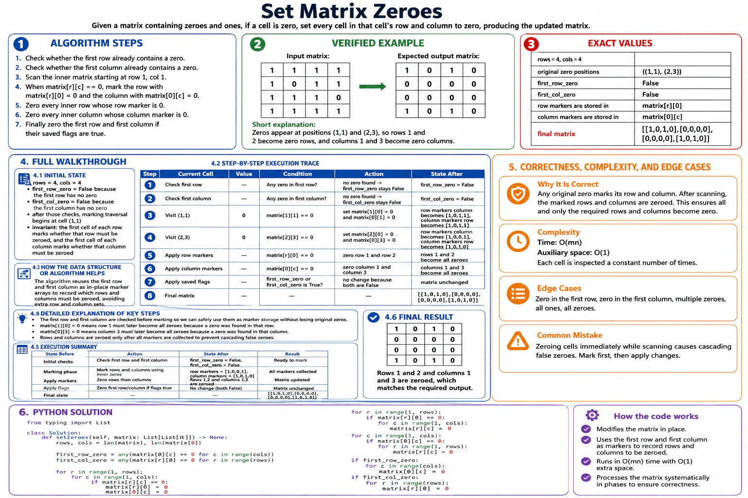
Set Matrix Zeroes diagram
How to Explain It in an Interview
1. Understand the input and required output

The input is a matrix containing zeroes and ones. We must update the same matrix. The function does not create or return a second matrix.

The example input is:

[[1, 1, 1, 1], [1, 0, 1, 1], [1, 1, 1, 0], [1, 1, 1, 1]]

The original zeroes are at positions (1,1) and (2,3). Therefore, rows 1 and 2 must become zero rows. Columns 1 and 3 must become zero columns.

The expected final matrix is:

[[1, 0, 1, 0], [0, 0, 0, 0], [0, 0, 0, 0], [1, 0, 1, 0]]

2. Save the first-row and first-column state

The first row and first column will be used as markers. Before changing them, we must remember whether they originally contain a zero.

In this example, the first row has no zero. Therefore, first_row_zero is False.

The first column also has no zero. Therefore, first_col_zero is False.

These flags preserve information that could otherwise be lost during marking.

3. Mark the required rows and columns

We scan the inner matrix starting at row 1 and column 1.

At cell (1,1), the value is

  1. The condition matrix[1][1] == 0 is true. We set matrix[1][0] = 0 to mark row
  2. We also set matrix[0][1] = 0 to mark column 1.

The row-marker column becomes [1,0,1,1]. The column-marker row becomes [1,0,1,1].

At cell (2,3), the value is 0. The condition matrix[2][3] == 0 is true. We set matrix[2][0] = 0 to mark row 2. We also set matrix[0][3] = 0 to mark column 3.

The row-marker column becomes [1,0,0,1]. The column-marker row becomes [1,0,1,0].

4. Apply the row and column markers

After the complete marking scan, we apply the row markers.

Because matrix[1][0] is 0, the inner cells of row 1 become zero. Because matrix[2][0] is 0, the inner cells of row 2 become zero.

Next, we apply the column markers.

Because matrix[0][1] is 0, the inner cells of column 1 become zero. Because matrix[0][3] is 0, the inner cells of column 3 become zero.

We collect all markers before applying them. This prevents newly written zeroes from creating false row or column markers.

5. Apply the saved flags

The saved flags control the complete first row and complete first column.

In this example, first_row_zero is False and first_col_zero is False. Therefore, the algorithm makes no additional change to the first row or first column.

The final matrix is:

[[1, 0, 1, 0], [0, 0, 0, 0], [0, 0, 0, 0], [1, 0, 1, 0]]

6. Explain why the result is correct

The first cell of each row records whether that row must become zero. The first cell of each column records whether that column must become zero.

Every original zero in the inner matrix creates both required markers. The algorithm applies the markers only after the scan is complete. Therefore, every required row and column becomes zero, while unrelated rows and columns remain unchanged.

The two saved flags correctly handle original zeroes in the first row or first column.

7. Explain the Python implementation and complexity

The code follows the same phases as the diagram. It saves the two flags, marks rows and columns, applies row markers, applies column markers, and finally applies the saved flags.

If the matrix has m rows and n columns, the code inspects cells a constant number of times. The time complexity is O(mn).

The code stores only two Boolean flags and loop variables. It reuses the matrix for markers, so the auxiliary space complexity is O(1).

Relevant edge cases are a zero in the first row, a zero in the first column, multiple zeroes, all ones, and all zeroes.

Key Insight / Why This Solution Works

The key insight is to reuse the first row and first column as in-place marker arrays. matrix[r][0] records whether row r must become zero. matrix[0][c] records whether column c must become zero. Before using these cells as markers, the algorithm saves whether the first row and first column originally contain a zero. The central invariant is that, after the marking scan, every required inner row and column has a zero marker. The algorithm then applies all row markers, all column markers, and finally the two saved flags.

Code
from typing import List


class Solution:
    def setZeroes(self, matrix: List[List[int]]) -> None:
        # Read the matrix dimensions.
        rows, cols = len(matrix), len(matrix[0])

        # Save whether the first row originally contains a zero.
        first_row_zero = any(matrix[0][c] == 0 for c in range(cols))

        # Save whether the first column originally contains a zero.
        first_col_zero = any(matrix[r][0] == 0 for r in range(rows))

        # Scan the inner matrix and store row and column markers.
        for r in range(1, rows):
            for c in range(1, cols):
                if matrix[r][c] == 0:
                    # Mark row r in the first column.
                    matrix[r][0] = 0

                    # Mark column c in the first row.
                    matrix[0][c] = 0

        # Zero every marked inner row.
        for r in range(1, rows):
            if matrix[r][0] == 0:
                for c in range(1, cols):
                    matrix[r][c] = 0

        # Zero every marked inner column.
        for c in range(1, cols):
            if matrix[0][c] == 0:
                for r in range(1, rows):
                    matrix[r][c] = 0

        # Zero the first row if it originally contained a zero.
        if first_row_zero:
            for c in range(cols):
                matrix[0][c] = 0

        # Zero the first column if it originally contained a zero.
        if first_col_zero:
            for r in range(rows):
                matrix[r][0] = 0


if __name__ == "__main__":
    example = [
        [1, 1, 1, 1],
        [1, 0, 1, 1],
        [1, 1, 1, 0],
        [1, 1, 1, 1],
    ]

    Solution().setZeroes(example)
    print(example)

    # Expected output:
    # [[1, 0, 1, 0],
    #  [0, 0, 0, 0],
    #  [0, 0, 0, 0],
    #  [1, 0, 1, 0]]
Time & Space Complexity

Let m be the number of rows and n be the number of columns. The algorithm performs several passes over parts of the matrix. Each cell is inspected only a constant number of times, so the total time complexity is O(mn). Auxiliary space means extra memory used by the algorithm. The solution stores only two Boolean flags and loop variables. It reuses the first row and first column as markers, so the auxiliary space complexity is O(1).

Where it is used

This in-place marker pattern is useful when a grid must be updated from row and column conditions while extra memory should remain constant. Similar ideas can be used in spreadsheet transformations, image masks, board-processing logic, and memory-limited matrix algorithms where part of the input can safely store temporary state.

Why Interviewers Ask This

This question tests whether a candidate can modify data in place without losing information that is still needed. It checks matrix traversal, update ordering, and invariant design. The interviewer also wants to see whether the candidate handles the special first row and first column correctly, avoids cascading updates, writes accurate Python loops, considers relevant edge cases, and explains why the solution takes O(mn) time with O(1) auxiliary space.

Common interview mistakes

A common mistake is zeroing cells immediately during the first scan. This creates cascading false zeroes and can change rows or columns that should remain unchanged. Another mistake is using the first row and first column as markers without first saving whether they originally contained a zero. Candidates may also reverse the marker roles by confusing matrix[r][0] with matrix[0][c]. Another error is applying markers before the full marking scan is complete. Finally, candidates may claim O(m+n) auxiliary space even though this in-place version uses O(1).

Interview tip

Explain the two saved flags before writing the loops. Then state the invariant clearly: the first column stores row markers, and the first row stores column markers. This makes the update order and correctness easier to justify.

Interviewer may ask next
How would the solution change if O(m+n) auxiliary space were allowed?

We could use one set for row indices and one set for column indices. During the first scan, we would add the row and column of every original zero. During a second scan, we would set matrix[r][c] to zero when r is in the row set or c is in the column set. This remains correct because the sets contain every row and column that had an original zero. The time complexity stays O(mn). The auxiliary space becomes O(m+n). The tradeoff is simpler update logic but higher memory use.

Why must the first row and first column be checked before they are used as markers?

Their cells may change during the marking phase. Without saved flags, we could not tell whether the first row or first column contained an original zero or only received a marker later. The flags preserve the original information. Correctness is maintained because the algorithm applies those flags only after all inner row and column updates. The time complexity remains O(mn), and the auxiliary space remains O(1).

16. Reverse nodes in a linked list in groups of k.CodingHardMicrosoft

Question Details

Given a linked-list head and a positive integer k, reverse the nodes k at a time. A final group containing fewer than k nodes must remain in its original order.

Short Interview Answer (30-60 seconds)

I use an iterative in-place solution with a dummy node. The dummy node makes it easy to reconnect the first reversed group. For each group, I move k steps to find its last node. If fewer than k nodes remain, I stop. Otherwise, I save the next part of the list, reverse exactly k nodes, reconnect the group, and continue from its new tail. The solution runs in O(n) time and uses O(1) auxiliary space.

Detailed Explanation

See the Code while reading this explanation.

The problem asks us to reverse a linked list in complete groups of k nodes. A final group with fewer than k nodes must keep its original order. The main challenge is changing node references without losing the remaining list. The selected solution uses a dummy node and reverses each complete group in place.

Useful Questions to Ask the Interviewer
  1. What input sizes, value ranges, and edge cases should the solution handle?
  2. What output should be returned for empty, invalid, or duplicate input?
  3. Should I prioritize execution time or memory use, and may I use the standard library?
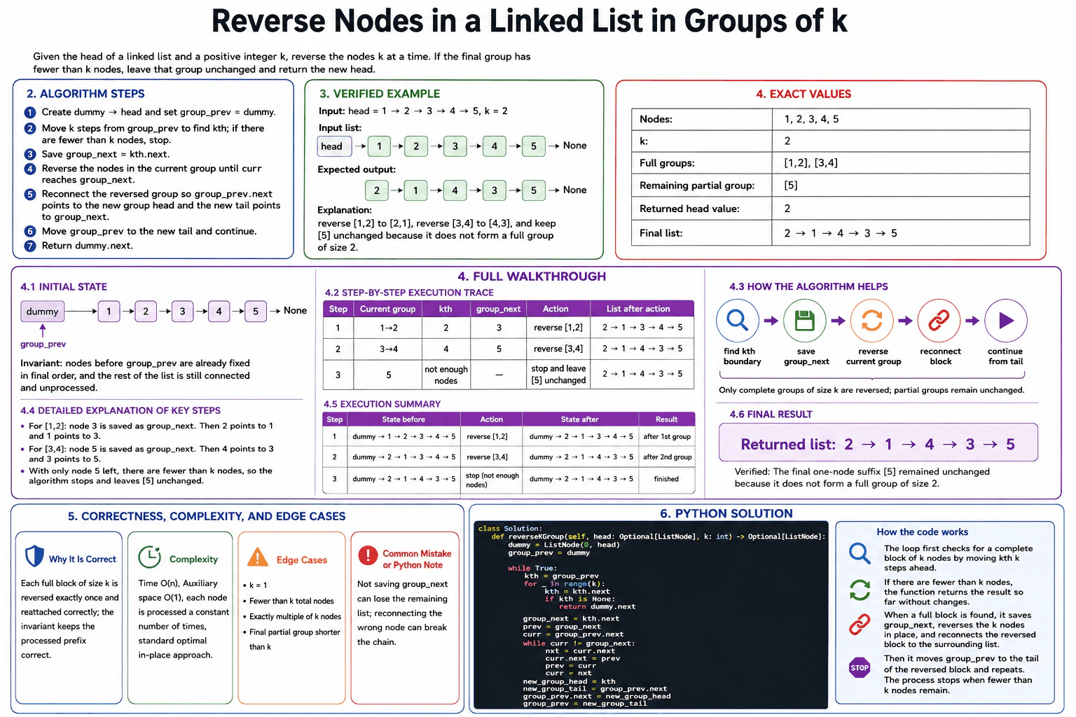
Reverse nodes in a linked list in groups of k. diagram
How to Explain It in an Interview
1. Understand the input and required output

The input is the head of a linked list and a positive integer k.

For the diagram example, the input is:

1 → 2 → 3 → 4 → 5

The value of k is 2.

We reverse every complete group of two nodes. The expected result is:

2 → 1 → 4 → 3 → 5

The final node 5 stays unchanged because it does not form a complete group of size 2.

2. Choose the in-place linked-list method

I place a dummy node before the real head. This makes it easy to reconnect the first reversed group because the head of the list may change.

I use group_prev to point to the node immediately before the group that I want to reverse.

The main invariant is that all nodes before group_prev are already in their final order. The remaining part of the list is still connected and has not been processed.

3. Confirm that a complete group exists

I start at group_prev and move k steps to find kth, the last node in the next group.

If kth becomes None before I finish k steps, fewer than k nodes remain. I return dummy.next immediately. This leaves the incomplete final group unchanged.

If a complete group exists, I save group_next = kth.next. This is the first node after the group. Saving it prevents the rest of the list from being lost during pointer changes.

4. Walk through the example

The initial list is:

dummy → 1 → 2 → 3 → 4 → 5

The pointer group_prev starts at dummy.

For the first group, the nodes are 1 and 2. The kth node is 2, and group_next is node 3.

I save node 3. I then reverse the group so node 2 points to node 1, and node 1 points to node 3.

The list becomes:

2 → 1 → 3 → 4 → 5

Node 1 was the old group head. It is now the group tail, so I move group_prev to node 1.

For the second group, the nodes are 3 and 4. The kth node is 4, and group_next is node 5.

I save node 5. I reverse the group so node 4 points to node 3, and node 3 points to node 5.

The list becomes:

2 → 1 → 4 → 3 → 5

I move group_prev to node 3, which is the new tail of that reversed group.

The next possible group contains only node 5. A complete group of two nodes does not exist, so processing stops. Node 5 remains unchanged.

5. Explain why the result is correct

Before each iteration, every node before group_prev is already in final order.

When a complete group of k nodes exists, the algorithm reverses exactly those k nodes. It connects the earlier part of the list to the new group head. It also connects the new group tail to group_next.

The list therefore stays connected. Each complete group is reversed exactly once. A final group with fewer than k nodes is never modified.

6. Explain the Python implementation

The code creates dummy and sets group_prev to dummy.

The outer loop first finds kth by moving forward k times. If kth becomes None, the function returns dummy.next.

For a complete group, the code saves group_next. It sets prev to group_next and curr to the first node in the current group.

The inner loop reverses one reference at a time until curr reaches group_next.

After the reversal, kth is the new group head. The old first node is the new group tail. The code connects group_prev to the new head and then moves group_prev to the new tail.

7. Explain complexity and edge cases

The time complexity is O(n). Each node is visited and rewired only a constant number of times.

The auxiliary space complexity is O(1). The algorithm uses only a fixed number of node references. It does not use an array, stack, or recursive call stack.

Important edge cases are k = 1, a list shorter than k, a list whose length is exactly divisible by k, and a list with a final incomplete group.

Key Insight / Why This Solution Works

The key idea is to reverse one complete group at a time without losing the remaining list. A dummy node is placed before the head so the first group can be handled like every later group. The pointer group_prev always points to the node before the current group. Before reversing, the algorithm confirms that k nodes exist and saves group_next, which is the first node after the group. The central invariant is that every node before group_prev is already in final order, while the remaining list is still connected and unprocessed.

Code
from __future__ import annotations

from dataclasses import dataclass
from typing import Optional


@dataclass
class ListNode:
    val: int
    next: Optional[ListNode] = None


class Solution:
    def reverseKGroup(self, head: Optional[ListNode], k: int) -> Optional[ListNode]:
        # Add a dummy node before the real head.
        # This makes the first reversed group easy to reconnect.
        dummy = ListNode(0, head)
        group_prev = dummy

        while True:
            # Find the kth node after group_prev.
            kth = group_prev
            for _ in range(k):
                kth = kth.next

                # Fewer than k nodes remain.
                # Return the list without changing the final partial group.
                if kth is None:
                    return dummy.next

            # Save the node after the group before changing any links.
            group_next = kth.next

            # Reverse the current group.
            # Starting prev at group_next connects the new tail correctly.
            prev = group_next
            curr = group_prev.next

            while curr != group_next:
                # Save the next node before reversing curr.next.
                nxt = curr.next

                # Reverse the current link.
                curr.next = prev

                # Move both working pointers forward.
                prev = curr
                curr = nxt

            # kth is the new head of the reversed group.
            new_group_head = kth

            # The old group head is now the new group tail.
            new_group_tail = group_prev.next

            # Connect the previous part to the new group head.
            group_prev.next = new_group_head

            # Continue from the tail of the reversed group.
            group_prev = new_group_tail


def build_linked_list(values: list[int]) -> Optional[ListNode]:
    # Build a linked list for the diagram example.
    dummy = ListNode(0)
    tail = dummy

    for value in values:
        tail.next = ListNode(value)
        tail = tail.next

    return dummy.next


def linked_list_to_list(head: Optional[ListNode]) -> list[int]:
    # Convert the result to a Python list for easy printing.
    values: list[int] = []
    curr = head

    while curr is not None:
        values.append(curr.val)
        curr = curr.next

    return values


if __name__ == "__main__":
    # Diagram input: 1 -> 2 -> 3 -> 4 -> 5, k = 2
    head = build_linked_list([1, 2, 3, 4, 5])

    result = Solution().reverseKGroup(head, 2)

    # Expected output: [2, 1, 4, 3, 5]
    print(linked_list_to_list(result))
Time & Space Complexity

The time complexity is O(n), where n is the number of nodes. Each node is checked and rewired only a constant number of times. The auxiliary space complexity is O(1). Auxiliary space means extra memory used by the algorithm. The solution uses only a fixed number of node references, so its extra memory does not grow with the list size.

Where it is used

This pattern is useful when linked-list records must be reordered in fixed-size blocks without copying them into another structure. It also teaches safe pointer updates, which are important in low-level data structures, queue implementations, memory-sensitive software, and other linked-list operations that modify nodes in place.

Why Interviewers Ask This

Interviewers use this problem to test whether a candidate can safely change linked-list references while keeping the list connected. They want to see correct boundary handling for the first group and the final incomplete group. The problem also tests the use of a dummy node, maintenance of an invariant, separation of group detection from group reversal, careful temporary-pointer updates, and accurate analysis of O(n) time and O(1) auxiliary space.

Common interview mistakes

A common mistake is changing node references before saving group_next. This can lose the remaining part of the list. Another mistake is connecting group_prev to the wrong node after reversal. Some candidates move group_prev to the new group head instead of the new group tail. Others reverse the final incomplete group even though it must stay unchanged. A final mistake is claiming that the iterative solution uses O(n) extra space when it actually uses O(1) auxiliary space.

Interview tip

Before writing the reversal loop, name the three group boundaries clearly: group_prev, kth, and group_next. Explain that group_next must be saved before any link changes. This makes the pointer updates easier to verify and prevents the rest of the list from being lost.

Interviewer may ask next
How would the solution change if the final group with fewer than k nodes also had to be reversed?

The stopping rule would change. Instead of returning immediately when fewer than k nodes remain, the algorithm would reverse all remaining nodes. It would still save the node after the group, which would be None for the final group. The pointer-reversal logic would remain similar. Every remaining node would then be included in the last reversal. The time complexity would stay O(n), and the auxiliary space would stay O(1). The tradeoff is that the final partial group would no longer preserve its original order.

Could this problem be solved recursively, and what would the tradeoff be?

Yes. A recursive solution can first confirm that k nodes exist, reverse the first k nodes, and recursively process the remaining list. The tail of the reversed group then points to the head returned by the recursive call. The time complexity remains O(n). The auxiliary space becomes O(n/k) because each complete group adds one recursive call to the call stack. The iterative solution is preferred when O(1) auxiliary space is required.

17. Majority ElementCodingEasyMicrosoft

Question Details

Given an integer array, return the value that appears more than half the time.

Short Interview Answer (30-60 seconds)

I would use the Boyer-Moore Majority Vote algorithm. I keep a candidate and a count while reading the array from left to right. When count is zero, the current number becomes the candidate. A matching number increases count, while a different number decreases it. These opposite votes cancel each other. Because the majority value appears more than half the time, it survives all cancellations. The algorithm runs in O(n) time and uses O(1) auxiliary space.

Detailed Explanation

See the Code while reading this explanation.

The problem asks us to return the value that appears more than half the time in an integer array. The Boyer-Moore Majority Vote algorithm fits this problem because it finds the majority without storing a frequency map. It keeps one candidate and one vote count. Different values cancel votes, but the true majority cannot be completely canceled.

Useful Questions to Ask the Interviewer
  1. What input sizes, value ranges, and edge cases should the solution handle?
  2. What output should be returned for empty, invalid, or duplicate input?
  3. Should I prioritize execution time or memory use, and may I use the standard library?
Majority Element diagram
How to Explain It in an Interview
1. Understand the input and output

The input is an integer array. The required output is the majority value, not an index or a count.

The example is [2, 2, 1, 1, 1, 2, 2]. The value 2 appears 4 times. The array has 7 elements, and half of 7 is 3.5. Because 4 is greater than 3.5, the correct output is 2.

The solution relies on the stated guarantee that a majority element exists.

2. Keep a candidate and a vote balance

I use two variables: candidate and count.

The candidate is the value that currently has unmatched support. The count is its net vote balance. A matching value adds one vote. A different value removes one vote.

The central invariant is that count tracks the unmatched votes for the current candidate among the values processed so far.

3. Initialize the state

I start with candidate = None and count = 0. Traversal begins at index 0.

When count is zero, there is no unmatched candidate vote. Therefore, the current number can become the new candidate, and count becomes 1.

4. Walk through the example

At index 0, the value is 2. The state is candidate = None and count = 0. Since count is zero, I choose 2 as the candidate and set count to 1.

At index 1, the value is 2. It matches candidate 2, so count increases from 1 to 2.

At index 2, the value is 1. It differs from candidate 2, so count decreases from 2 to 1.

At index 3, the value is 1. It differs again, so count decreases from 1 to 0. The two earlier votes for 2 have now been canceled by two votes for 1.

At index 4, the value is 1. Since count is zero, I choose 1 as the new candidate and set count to 1.

At index 5, the value is 2. It differs from candidate 1, so count decreases from 1 to 0.

At index 6, the value is 2. Since count is zero, I choose 2 as the candidate and set count to 1.

All 7 elements are processed. The final candidate is 2, so the function returns 2.

5. Explain why the algorithm is correct

Each decrement pairs one occurrence of the current candidate with one different value. The pair cancels out.

The true majority appears more than half the time. This means it appears more often than all other values combined. Therefore, the other values cannot cancel every occurrence of the majority. The majority must remain as the final surviving candidate.

6. Explain the Python implementation

The function receives nums, which is a list of integers. It initializes candidate to None and count to 0.

The loop processes each number from left to right. If count is zero, it starts a new candidate. If the number matches the candidate, it increases count. Otherwise, it decreases count.

After the loop, it returns the surviving candidate.

7. Explain complexity and edge cases

The algorithm processes each array element once, so its time complexity is O(n).

It stores only candidate, count, and the current number. Its auxiliary space complexity is O(1).

Relevant edge cases include a one-element array, negative values, zero values, many duplicates, and a majority that appears mainly near the end of the array.

Key Insight / Why This Solution Works

The key idea is pairwise vote cancellation. The algorithm stores a current candidate and a count. When the current value matches the candidate, count increases. When it differs, count decreases. A decrease represents canceling one candidate occurrence with one opposing occurrence. When count becomes zero, the earlier processed values contain no unmatched support for the old candidate, so the next value starts as a new candidate. The invariant is that count equals the net unmatched vote balance for candidate. Since the majority value appears more than all other values combined, it cannot be fully canceled and must be the final candidate.

Code
from typing import List


class Solution:
    def majorityElement(self, nums: List[int]) -> int:
        # Start with no active candidate and no unmatched votes.
        candidate = None
        count = 0

        # Process each number from left to right.
        for num in nums:
            # If all earlier votes are canceled, start a new candidate.
            if count == 0:
                candidate = num
                count = 1
            # A matching value adds one vote for the candidate.
            elif num == candidate:
                count += 1
            # A different value cancels one candidate vote.
            else:
                count -= 1

        # The problem guarantees that a majority element exists.
        return candidate


if __name__ == "__main__":
    nums = [2, 2, 1, 1, 1, 2, 2]
    result = Solution().majorityElement(nums)
    print(result)  # Expected output: 2
Time & Space Complexity

The time complexity is O(n), where n is the number of elements in the array. The loop moves from left to right and processes each element once. The auxiliary space complexity is O(1). Auxiliary space means extra memory used by the algorithm. Only candidate, count, and the current loop value are stored, so the extra memory stays constant even when the input becomes larger.

Where it is used

This pattern is useful when one value is guaranteed to occur more than half the time and memory must stay small. It can identify a dominant vote, repeated event type, sensor reading, status code, or category in a large collection or stream. It avoids the extra memory required by a full frequency dictionary.

Why Interviewers Ask This

Interviewers use this problem to test whether you recognize the Boyer-Moore cancellation pattern instead of immediately building a frequency map. They want to see whether you can maintain a small state, explain the invariant, handle candidate resets correctly, and prove why the majority survives. They also evaluate whether your Python code handles duplicates, negative values, and zero values, and whether you correctly state O(n) time and O(1) auxiliary space.

Common interview mistakes

One mistake is treating count as the candidate's total frequency. It is only the net vote balance after cancellations. Another mistake is changing candidate whenever a different value appears. Candidate changes only when count is zero. Candidates may also forget to set count to 1 after choosing a new candidate. Some return count instead of candidate. Others claim the algorithm verifies the candidate's real frequency, but this single pass depends on the guarantee that a majority exists. It is also incorrect to claim that the algorithm uses O(n) extra space.

Interview tip

Explain the meaning of count before writing the loop: it is the candidate's net unmatched vote balance, not its total frequency. Then trace every point where count reaches zero and a new candidate is selected.

Interviewer may ask next
What changes if a majority element is not guaranteed to exist?

The first Boyer-Moore pass still produces a candidate, but that candidate may not be a true majority. I would make a second pass and count its occurrences. I would return it only if its frequency is greater than n divided by 2. Otherwise, I would return None or another required fallback. Correctness is preserved because the second pass verifies the majority condition directly. The total time remains O(n), and auxiliary space remains O(1). The tradeoff is one additional pass.

Can the algorithm work when the numbers arrive as a stream?

Yes. The candidate-selection pass works with streaming input because each new number updates only candidate and count. Processing n values takes O(n) total time and O(1) auxiliary space. If a majority is guaranteed, the final candidate can be returned. If a majority is not guaranteed, verification needs another pass or stored frequency information. A one-pass stream may not allow that verification, which is the main tradeoff.

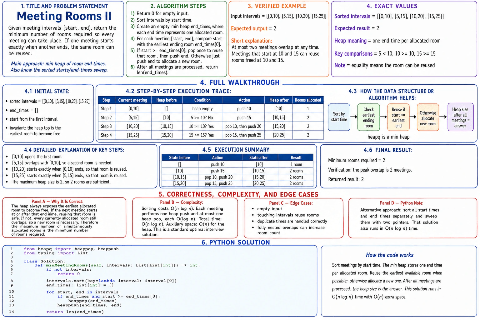
18. Meeting Rooms IICodingMediumMicrosoft

Question Details

Given meeting intervals, return the minimum number of rooms required so every meeting can take place. Discuss both a priority-queue solution and a sorted start-times/end-times solution.

Short Interview Answer (30-60 seconds)

I would sort the meetings by start time and keep a min heap of room end times. The smallest end time represents the room that becomes available first. For each meeting, I reuse that room when the meeting starts at or after the earliest end time. Otherwise, I allocate another room. I then push the current end time. The final heap size is the minimum number of rooms required. The time complexity is O(n log n), and the auxiliary space is O(n).

Detailed Explanation

See the Code while reading this explanation.

The problem asks for the minimum number of rooms needed for all meetings. A room can be reused when a new meeting starts exactly when an earlier meeting ends. I sort the meetings by start time and use a min heap. The heap stores one end time for each allocated room and exposes the room that becomes available first.

Useful Questions to Ask the Interviewer
  1. What input sizes, value ranges, and edge cases should the solution handle?
  2. What output should be returned for empty, invalid, or duplicate input?
  3. Should I prioritize execution time or memory use, and may I use the standard library?
Meeting Rooms II diagram
How to Explain It in an Interview
1. Understand the input and required output

The input is a list of meeting intervals. Each interval has the form [start, end). The start time is included. The end time is when the room becomes free.

The output is one integer. It is the minimum number of rooms needed so that overlapping meetings do not use the same room.

For the example [[0,10], [5,15], [10,20], [15,25]], the expected output is 2.

2. Choose the algorithm and data structure

I first sort the intervals by start time. This lets me process meetings in the order they begin.

I use a min heap named end_times. Each heap entry is the end time currently associated with one allocated room. The smallest end time is at the top. It tells me which allocated room becomes available first.

The question also asks about the sorted start-times and end-times solution. That is another valid O(n log n) approach. The diagram uses the min-heap solution as the main implementation.

3. Initialize the state

After sorting, the intervals are [[0,10], [5,15], [10,20], [15,25]].

The heap starts empty:

end_times = []

The central invariant is that every heap entry represents one allocated room. The heap top gives the earliest end time among those rooms.

4. Walk through the example

For [0,10], the heap is empty. I allocate the first room and push 10. The heap changes from [] to [10]. The room count is 1.

For [5,15], the heap is [10]. I check whether 5 >= 10. The condition is false. The earliest room is still busy, so I allocate a second room and push 15. The heap changes to [10,15]. The room count is 2.

For [10,20], the heap is [10,15]. I check whether 10 >= 10. The condition is true. The meeting starting at 10 can reuse the room that becomes free at 10. I pop 10 and push 20. The heap changes to [15,20]. The room count remains 2.

For [15,25], the heap is [15,20]. I check whether 15 >= 15. The condition is true. I pop 15 and push 25. The heap changes to [20,25]. The room count remains 2.

After all four meetings are processed, the heap contains two entries. The returned result is 2.

5. Explain why the result is correct

The heap always exposes the allocated room with the earliest end time. If the next meeting starts at or after that time, reusing the room is safe because the earlier meeting has finished.

If the next meeting starts before the earliest end time, every allocated room is still busy at that start time. A new room is therefore necessary.

The code pops at most one end time because one new meeting can reuse only one room. Each heap entry represents one allocated room, so the final heap size is the minimum number of rooms required.

6. Explain the Python implementation

The function first returns 0 for empty input. It then sorts the intervals using each interval's start time.

For every meeting, the code compares its start time with the smallest end time in the heap. If the start time is at least that end time, the code pops the end time and reuses that room. It then pushes the current meeting's end time.

After all meetings are processed, the function returns len(end_times).

7. Explain complexity and edge cases

Sorting takes O(n log n) time. Every meeting causes one heap push and at most one heap pop. Each heap operation takes O(log n), so the total time is O(n log n).

The heap can contain up to n end times, so the auxiliary space is O(n).

Important edge cases are empty input, meetings that touch at the same time, duplicate start or end times, and fully overlapping or nested meetings.

Key Insight / Why This Solution Works

The key insight is to process meetings in start-time order and always inspect the allocated room with the earliest end time. A min heap keeps the smallest end time at the top. Each heap value represents one allocated room. If the next meeting starts at or after the smallest end time, that room can be reused. Otherwise, every allocated room is still busy, so another room is needed. The invariant is that every heap entry represents one allocated room and the heap top gives the earliest room-release time.

Code
from heapq import heappop, heappush
from typing import List


class Solution:
    def minMeetingRooms(self, intervals: List[List[int]]) -> int:
        # Step 1: Empty input needs no rooms.
        if not intervals:
            return 0

        # Step 2: Process meetings in the order they start.
        intervals.sort(key=lambda interval: interval[0])

        # Each heap value is the end time associated with one allocated room.
        # The smallest end time is always at index 0.
        end_times: list[int] = []

        # Step 3: Process every meeting.
        for start, end in intervals:
            # Reuse the room with the earliest end time when possible.
            # Equality is allowed because a meeting can start exactly
            # when another meeting ends.
            if end_times and start >= end_times[0]:
                heappop(end_times)

            # Push the current meeting's end time.
            # This represents either a reused room or a new room.
            heappush(end_times, end)

        # One heap entry represents one allocated room.
        return len(end_times)


if __name__ == "__main__":
    example_intervals = [[0, 10], [5, 15], [10, 20], [15, 25]]
    result = Solution().minMeetingRooms(example_intervals)
    print(result)  # Expected output: 2
Time & Space Complexity

Let n be the number of meetings. Sorting the meetings costs O(n log n). Each meeting is pushed into the min heap once. A meeting may also cause one pop when a room is reused. A heap push or pop costs O(log n), so the total time is O(n log n). The heap may contain up to n end times when many meetings overlap. Therefore, the auxiliary space is O(n).

Where it is used

This pattern is useful in scheduling systems. Examples include meeting-room booking, classroom allocation, worker scheduling, server-job assignment, and finding the maximum number of tasks that run at the same time. A min heap is useful when software must quickly find the resource that becomes available first.

Why Interviewers Ask This

This question tests whether you can recognize an interval-overlap problem and choose a suitable data structure. The interviewer wants to see whether you understand sorting order, min-heap operations, and the rule for meetings that touch at the same time. It also tests whether you can maintain a clear invariant, trace state changes correctly, compare the heap method with the sorted starts-and-ends method, and explain O(n log n) time and O(n) auxiliary space accurately.

Common interview mistakes

A common mistake is using start > earliest_end instead of start >= earliest_end. Equality must allow room reuse. Another mistake is forgetting to sort the intervals by start time. Some candidates use a max heap instead of a min heap, so they cannot quickly find the earliest available room. Others return the largest heap size seen even though this exact implementation keeps one entry per allocated room and returns the final heap size. It is also incorrect to ignore the sorting cost or claim O(1) auxiliary space.

Interview tip

State the heap invariant before writing code: each heap entry represents one allocated room, and the heap top gives the earliest end time. Then explain that start >= end_times[0] is the exact condition for safely reusing a room.

Interviewer may ask next
How would you solve this using sorted start times and end times instead of a heap?

Create one sorted list of all start times and one sorted list of all end times. Use a start pointer and an end pointer. If the next start is before the next end, a new meeting becomes active, so increase the active-room count and move the start pointer. Otherwise, a meeting has ended, so decrease the active count and move the end pointer. When start equals end, process the end first so the room can be reused. Track the maximum active count. The time complexity is O(n log n), and the auxiliary space is O(n) for the two sorted lists.

What changes if meetings arrive as a stream?

The heap method can work when meetings arrive in nondecreasing start-time order. In that version, keep a min heap of active meeting end times. Before adding a new meeting, pop every end time that is less than or equal to its start time. Then push the new end time and update the largest heap size seen. Removing all expired meetings is needed because this streaming version makes the heap represent active meetings. Each meeting causes O(log n) amortized heap work, and the heap uses O(n) space in the worst case.

19. Maximize a product after applying the same XOR value.CodingMediumMicrosoft

Question Details

Given positive integers a, b, and n, choose an integer x with 0 <= x < 2^n to maximize (a XOR x) * (b XOR x). Return the optimized product modulo 1,000,000,007.

Short Interview Answer (30-60 seconds)

I build the two XOR results directly instead of trying every possible x. First, I preserve the bits above the lowest n positions because x cannot change them. Then I process the allowed bits from high to low. Equal input bits let me set the bit in both results. Different bits give one result a 1, so I give it to the smaller current result. This keeps the values balanced and maximizes their product in O(n) time and O(1) auxiliary space.

Detailed Explanation

See the Code while reading this explanation.

The problem asks us to choose one integer x, where 0 <= x < 2^n, that maximizes (a XOR x) * (b XOR x). Trying every possible x would require up to 2^n attempts. The diagram uses a greedy bit-by-bit solution instead. It constructs the two final XOR values directly and processes the allowed bits from the most significant position to the least significant position.

Useful Questions to Ask the Interviewer
  1. What input sizes, value ranges, and edge cases should the solution handle?
  2. What output should be returned for empty, invalid, or duplicate input?
  3. Should I prioritize execution time or memory use, and may I use the standard library?
Maximize a product after applying the same XOR value. diagram
How to Explain It in an Interview
1. Understand what x can change

Because x is smaller than 2^n, it can contain 1 bits only in positions 0 through n - 1.

This means bits above position n - 1 cannot change in either a XOR x or b XOR x.

We return the maximum product modulo 1,000,000,007. We do not need to return x.

2. Initialize the two final values

We construct two values directly:

  • result_a represents a XOR x.
  • result_b represents b XOR x.

First, we create:

mask = (1 << n) - 1

This mask contains 1 in each of the lowest n positions.

We then preserve the higher bits:

  • result_a = a & ~mask
  • result_b = b & ~mask

The central invariant is that after each processed bit, the selected higher-bit prefixes form the best possible pair for maximizing the product.

3. Process bits from high to low

We examine positions from n - 1 down to 0.

At each position i, we read:

  • a_bit = (a >> i) & 1
  • b_bit = (b >> i) & 1

If a_bit equals b_bit, one choice of the shared x bit makes both XOR result bits equal to 1. Setting both bits to 1 increases both values, so it is always better than making both bits 0.

If a_bit and b_bit differ, the two XOR result bits must be one 1 and one

  1. We cannot make both of them
  2. We give the 1 to the smaller current result. This keeps the two values as balanced as possible and produces the larger product.
4. Walk through the verified example

The example uses:

  • a = 12 = 1100₂
  • b = 5 = 0101₂
  • n = 4
  • mask = 1111₂

There are no higher bits to preserve, so the initial state is:

  • result_a = 0
  • result_b = 0

We process bits 3, 2, 1, and 0.

At bit 3, a_bit is 1 and b_bit is 0. The bits differ. The state before the step is (0, 0). The values are tied, so the code's tie rule gives the 1 to result_b. The state becomes (0, 8). The selected x bit is 1.

At bit 2, both original bits are 1. The bits match, so we set bit 2 in both result values. The state changes from (0, 8) to (4, 12). The selected x bit is 0.

At bit 1, both original bits are 0. The bits match again, so we set bit 1 in both result values. The state changes from (4, 12) to (6, 14). The selected x bit is 1.

At bit 0, a_bit is 0 and b_bit is 1. The bits differ. result_a is smaller than result_b, so result_a receives the 1. The state changes from (6, 14) to (7, 14). The selected x bit is 1.

The selected bits give one optimal value:

x = 1011₂ = 11

The final calculation is:

  • 12 XOR 11 = 7
  • 5 XOR 11 = 14
  • 7 * 14 = 98

Therefore, the returned value is 98.

5. Explain why the greedy choice is correct

Bits above the lowest n positions cannot change, so the algorithm must preserve them.

When the two original bits match, both XOR result bits can become 1. This is always better than making both result bits 0.

When the original bits differ, that position must produce one 1 and one 0 across the two results. The total contribution from that position is fixed. Giving the 1 to the smaller current result keeps the values more balanced. For a fixed sum, a more balanced pair has a larger product.

We process higher bits first because they have a greater effect than lower bits. This lets each step choose the best possible prefix before moving to the next bit.

6. Explain the Python implementation

The code creates the mask and preserves all higher bits in result_a and result_b.

It then loops from bit n - 1 down to bit 0. For each position, it reads the corresponding bits from a and b.

When those bits match, it uses bitwise OR to set the current bit in both results.

When they differ, it compares the current partially built results. It sets the bit only in the smaller result. If the values are tied, the else branch gives the bit to result_b, matching the diagram.

After every allowed bit has been processed, the code multiplies result_a and result_b and applies modulo 1,000,000,007.

7. Explain complexity and edge cases

The loop processes n bit positions, so the time complexity is O(n).

The algorithm stores only a fixed number of integer variables. It does not use an array, map, stack, queue, or recursion. Therefore, the auxiliary space complexity is O(1).

If n is 0, the loop does not run. The mask is 0, x must be 0, and the original values remain unchanged.

Bits above the lowest n positions are always preserved.

If a equals b, equal bit choices are applied to both results, so the two constructed values remain equal.

The modulo operation is applied only to the final product.

Key Insight / Why This Solution Works

The solution uses a greedy bit-by-bit approach. It constructs a XOR x and b XOR x directly. Bits above the lowest n positions are copied first because x cannot change them. The remaining bits are processed from high to low. If the two original bits match, both result bits are set to 1. If they differ, exactly one result can receive 1, so the algorithm gives it to the smaller current result. The invariant is that after every step, the processed higher-bit prefixes form the best possible pair. This works because higher bits dominate lower bits, and balancing two values maximizes their product when the contribution at the current bit is fixed.

Code
class Solution:
    def maximumXorProduct(self, a: int, b: int, n: int) -> int:
        # The problem requires the final product modulo this value.
        MOD = 1_000_000_007

        # Create a mask with 1 in each of the lowest n bit positions.
        mask = (1 << n) - 1

        # Preserve all higher bits because x cannot change them.
        # result_a will become a XOR x.
        # result_b will become b XOR x.
        result_a = a & ~mask
        result_b = b & ~mask

        # Process allowed bits from most significant to least significant.
        for i in range(n - 1, -1, -1):
            # Numeric value of the current bit position.
            bit = 1 << i

            # Read bit i from a and b.
            a_bit = (a >> i) & 1
            b_bit = (b >> i) & 1

            if a_bit == b_bit:
                # Equal original bits can produce 1 in both XOR results.
                result_a |= bit
                result_b |= bit
            elif result_a < result_b:
                # Different original bits produce one 1 and one 0.
                # Give the 1 to the smaller current result.
                result_a |= bit
            else:
                # Give the 1 to result_b when it is smaller or tied.
                # This matches the tie behavior shown in the diagram.
                result_b |= bit

        # Apply modulo only after constructing both final values.
        return (result_a * result_b) % MOD


if __name__ == "__main__":
    # Verified example from the diagram.
    a = 12
    b = 5
    n = 4

    solution = Solution()
    result = solution.maximumXorProduct(a, b, n)

    print(result)  # Expected output: 98
Time & Space Complexity

The time complexity is O(n) because the loop visits each of the n allowed bit positions once. Each iteration performs only a fixed number of shifts, bit operations, comparisons, and assignments. The auxiliary space complexity is O(1). Auxiliary space means extra memory used by the algorithm. The code stores only a mask, two result values, the current bit position, and a few temporary integers. This memory does not grow with n.

Where it is used

This greedy bit pattern is useful when one shared bitmask changes two integers and the goal is to maximize a numeric expression. Similar reasoning appears in bitmask optimization, compact flags, integer encoding, low-level permissions, and interview problems where high-order bit decisions must be made before lower-order decisions.

Why Interviewers Ask This

This problem tests whether a candidate can reason about XOR and binary positions instead of using brute force. The interviewer is checking whether the candidate understands how one shared x bit affects both values, why high bits must be processed first, and why balancing two numbers increases their product. It also evaluates greedy reasoning, maintenance of a clear invariant, correct use of Python bitwise operations, handling of edge cases, and accurate O(n) time and O(1) auxiliary-space analysis.

Common interview mistakes

One mistake is comparing only the original values a and b when deciding which result receives a differing bit. The algorithm must compare the current partially built result_a and result_b. Another mistake is processing bits from low to high. The code must process high bits first because they have the greatest effect. Candidates may also forget to preserve bits above the lowest n positions. Another error is trying to set both result bits to 1 when the original bits differ, which one shared x bit cannot do. A final mistake is applying modulo before making greedy comparisons. Modulo should be applied only to the returned product.

Interview tip

State the invariant before coding: after each high-to-low step, the processed prefixes are the best possible prefixes. Then explain the two cases separately. Equal bits make both results gain a 1. Different bits give the 1 to the smaller current result.

Interviewer may ask next
How would you also return one optimal value of x?

Add an integer variable x and start it at 0. At every bit position, record the x bit that creates the chosen result bits. When the original bits match, use x_bit = 1 - a_bit so both XOR result bits become 1. When the bits differ, the result that receives the 1 determines whether x_bit is 0 or 1. Set bit i in x when the selected x bit is 1. The greedy choices and correctness proof do not change. The time complexity remains O(n), and the auxiliary space remains O(1).

Why can we not simply give every differing bit to the same result?

Giving every differing bit to the same result can make one value much larger and the other much smaller. The contribution of each differing bit is split as one 1 and one 0, so assigning the 1 to the smaller current result keeps the pair balanced. A balanced pair has a larger product when its total contribution is fixed. The same high-to-low greedy algorithm is still used, with O(n) time and O(1) auxiliary space.

20. Maximize added edges subject to special-employee connection limits.CodingHardMicrosoft

Question Details

You are given employees connected by an undirected graph, a set of special employees, and a limit on how many special employees any employee may be connected to. Add the maximum possible number of valid new edges without self-edges, duplicate edges, or violating the limit.

Short Interview Answer (30-60 seconds)

I split the missing edges into three groups. First, I add every missing edge between non-special employees because those edges never increase a special-neighbor count. Next, I greedily connect each non-special employee to special employees until that employee reaches its limit. Finally, I use memoized DFS for missing special-to-special edges because each selected edge uses capacity from both special endpoints. The total time is O(n^2 + q · 2^q), and the auxiliary space is O(n^2 + 2^q).

Detailed Explanation

See the Code while reading this explanation.

The problem asks for the largest number of new undirected edges we can add. We cannot add self-edges or duplicate edges. After every addition, no employee may have more than limit directly adjacent special employees. The solution separates missing edges into three types. Two types can be handled greedily. The remaining special-to-special edges need an exact memoized DFS because their choices share endpoint capacity.

Useful Questions to Ask the Interviewer
  1. What input sizes, value ranges, and edge cases should the solution handle?
  2. What output should be returned for empty, invalid, or duplicate input?
  3. Should I prioritize execution time or memory use, and may I use the standard library?
Maximize added edges subject to special-employee connection limits. diagram
How to Explain It in an Interview
1. Understand the input and required output

The input contains n employees numbered from 0 to n - 1, a list of existing undirected edges, a set of special employees, and an integer limit.

For each employee, we count how many directly adjacent employees are special. This count must never be greater than limit.

The output is one integer. It is the maximum number of valid new edges that can be added.

2. Build the graph state

The code builds an adjacency matrix named adj.

adj[u][v] is True when employees u and v already have an edge. Because the graph is undirected, the code updates both adj[u][v] and adj[v][u].

The code also builds neighbor sets. These sets are used to calculate special_deg[u].

special_deg[u] is the number of special employees directly adjacent to employee u.

For the example:

  • n = 6
  • special = {0, 2}
  • limit = 1
  • existing edges are (0,1), (1,3), and (2,4)

The initial state is:

special_deg = [0, 1, 0, 0, 1, 0]

The non-special employees are [1, 3, 4, 5]. The special employees are [0, 2].

3. Add all missing non-special-to-non-special edges

An edge between two non-special employees does not increase either endpoint's number of special neighbors. Therefore, every missing edge of this type is safe.

Among employees {1,3,4,5}, edge (1,3) already exists. The code adds the five missing edges:

(1,4), (1,5), (3,4), (3,5), (4,5)

The added count becomes 5.

The special_deg array remains:

[0, 1, 0, 0, 1, 0]

4. Fill each non-special employee's remaining limit

The code visits non-special employees in the order [1,3,4,5]. For each one, it tries the sorted special employees [0,2].

Employee 1 already has one special neighbor, employee 0. The limit is 1, so the code adds nothing.

Employee 3 has zero special neighbors. The code adds (0,3). The added count becomes 6, and special_deg[3] becomes 1.

The state becomes:

special_deg = [0, 1, 0, 1, 1, 0]

Employee 4 already has one special neighbor, employee 2. The code adds nothing.

Employee 5 has zero special neighbors. The code adds (0,5). The added count becomes 7, and special_deg[5] becomes 1.

The state becomes:

special_deg = [0, 1, 0, 1, 1, 1]

These choices are independent for non-special employees. A special-to-non-special edge increases only the non-special endpoint's number of special neighbors. The special endpoint gains a non-special neighbor, so its special-neighbor count does not change.

5. Search the missing special-to-special edges

A special-to-special edge increases the special-neighbor count of both endpoints. This means candidate edges can compete for the same remaining capacity.

The code calculates each special employee's remaining capacity:

cap[s] = limit - special_deg[s]

Before the DFS:

  • cap[0] = 1
  • cap[2] = 1

The only missing special-to-special edge is (0,2).

The memoized DFS considers two choices for each candidate edge:

  • skip the edge
  • take the edge when both endpoints still have capacity

The DFS takes (0,2). Both capacities become zero. The added count becomes 8.

After adding (0,2), the final special-neighbor counts are:

[1, 1, 1, 1, 1, 1]

The algorithm stops and returns 8.

6. Explain why the result is correct

The central invariant is:

special_deg[u] <= limit

The first phase is safe because an edge between two non-special employees does not change any special-neighbor count.

The second phase is correct because each non-special employee can be filled independently. The code stops adding special neighbors to that employee when its count reaches limit.

The third phase is correct because the DFS considers every feasible take-or-skip combination of missing special-to-special edges. It takes an edge only when both special endpoints have remaining capacity.

Therefore, the algorithm adds every always-safe edge and finds the maximum feasible number of coupled special-to-special edges.

One valid final added-edge set is:

{(1,4), (1,5), (3,4), (3,5), (4,5), (0,3), (0,5), (0,2)}

7. Explain complexity and edge cases

Building the adjacency matrix and running the greedy phases take O(n^2) time.

Let q be the number of missing edges between special employees. The exact memoized DFS has the stated cost O(q · 2^q).

The full time complexity is:

O(n^2 + q · 2^q)

The auxiliary space complexity is:

O(n^2 + 2^q)

The adjacency matrix uses O(n^2) space. The memoized special-only search uses exponential space in the stated analysis.

Important edge cases are limit = 0, employees already at the limit, no missing edges, zero special employees, and one special employee.

Key Insight / Why This Solution Works

The key insight is to divide missing edges by endpoint type. Missing edges between two non-special employees are always safe, so the algorithm adds all of them. Missing edges between one non-special and one special employee can be handled independently for each non-special employee, so the algorithm greedily fills that employee's remaining limit. Missing edges between two special employees are coupled because each chosen edge consumes one capacity unit from both endpoints. The algorithm solves only that smaller coupled part with take-or-skip DFS and memoization. The invariant is that special_deg[u] never exceeds limit.

Code
from functools import lru_cache
from typing import List, Set, Tuple


def max_added_edges(
    n: int,
    edges: List[Tuple[int, int]],
    special: Set[int],
    limit: int,
) -> int:
    # Store special employees in a set for fast membership checks.
    special = set(special)

    # adj[u][v] is True when the undirected edge (u, v) exists.
    # The matrix lets us check for duplicate edges directly.
    adj = [[False] * n for _ in range(n)]

    # nbrs[u] stores the original neighbors of employee u.
    # We use it to calculate the initial special-neighbor counts.
    nbrs = [set() for _ in range(n)]

    # Load every original undirected edge in both directions.
    for u, v in edges:
        adj[u][v] = True
        adj[v][u] = True
        nbrs[u].add(v)
        nbrs[v].add(u)

    # special_deg[u] is the number of special neighbors of employee u.
    special_deg = [sum(1 for v in nbrs[u] if v in special) for u in range(n)]

    added = 0

    # Keep the traversal order used in the diagram.
    ordinary = [u for u in range(n) if u not in special]
    specials = sorted(special)

    # Phase 1:
    # Add every missing edge between two non-special employees.
    # These edges do not increase any special-neighbor count.
    for i in range(len(ordinary)):
        for j in range(i + 1, len(ordinary)):
            u = ordinary[i]
            v = ordinary[j]

            if not adj[u][v]:
                adj[u][v] = True
                adj[v][u] = True
                added += 1

    # Phase 2:
    # Fill each non-special employee's remaining special-neighbor limit.
    for u in ordinary:
        for s in specials:
            # Stop for this employee when its limit is reached.
            if special_deg[u] == limit:
                break

            # Add only a missing edge.
            if not adj[u][s]:
                adj[u][s] = True
                adj[s][u] = True
                special_deg[u] += 1
                added += 1

    # Phase 3:
    # A special-to-special edge consumes one capacity unit
    # from both special endpoints.
    caps = [limit - special_deg[s] for s in specials]

    # Store each missing special-to-special edge by the positions
    # of its endpoints inside the sorted specials list.
    candidates: List[Tuple[int, int]] = []
    for i in range(len(specials)):
        for j in range(i + 1, len(specials)):
            u = specials[i]
            v = specials[j]

            if not adj[u][v]:
                candidates.append((i, j))

    @lru_cache(maxsize=None)
    def dfs(pos: int, state: Tuple[int, ...]) -> int:
        # Base case: every candidate edge has been considered.
        if pos == len(candidates):
            return 0

        # Choice 1: skip the current candidate edge.
        best = dfs(pos + 1, state)

        i, j = candidates[pos]
        current_caps = list(state)

        # Choice 2: take the edge only if both endpoints have capacity.
        if current_caps[i] > 0 and current_caps[j] > 0:
            current_caps[i] -= 1
            current_caps[j] -= 1

            best = max(
                best,
                1 + dfs(pos + 1, tuple(current_caps)),
            )

        return best

    # Combine the two greedy phases with the exact special-only result.
    return added + dfs(0, tuple(caps))


if __name__ == "__main__":
    # Exact example from the diagram.
    n = 6
    edges = [(0, 1), (1, 3), (2, 4)]
    special = {0, 2}
    limit = 1

    result = max_added_edges(n, edges, special, limit)
    print(result)  # Expected output: 8
Time & Space Complexity

The adjacency matrix and the two greedy phases take O(n^2) time. Let q be the number of missing special-to-special edges. The memoized DFS considers take-or-skip choices for those edges, so the stated search cost is O(q · 2^q). The complete time complexity is O(n^2 + q · 2^q). The auxiliary space is O(n^2 + 2^q). The adjacency matrix uses O(n^2) memory. The cached DFS states use exponential memory for the special-only subproblem. This approach is practical when the number of special employees, and therefore q, is modest.

Where it is used

This pattern is useful when a graph problem contains many independent safe choices and a smaller group of choices that share limited resources. Similar cases appear when adding communication links, permissions, assignments, or relationships while enforcing per-user limits. The greedy phases handle choices that cannot hurt future choices. The exact search is used only for the smaller coupled part.

Why Interviewers Ask This

This question tests whether you can split a graph problem into independent and coupled choices. The interviewer wants to see a correct undirected graph representation, careful tracking of each employee's special-neighbor count, and a clear invariant. It also checks whether you can prove when greedy additions are safe, recognize when exact search is still needed, write consistent Python code, and state the exponential tradeoff honestly.

Common interview mistakes

A common mistake is treating every missing edge as independent. Special-to-special edges are coupled because both endpoints lose capacity. Another mistake is updating the special endpoint's count after adding a special-to-non-special edge. Only the non-special endpoint gains a special neighbor. Candidates may also forget to reject duplicate edges, update only one direction of an undirected edge, forget the DFS skip choice, calculate special capacities before finishing the greedy phase, or claim polynomial time even though the special-only search is exponential in q.

Interview tip

Explain the three edge types before writing code. Say which type is always safe, which type can be handled independently, and which type shares capacity. This makes the reason for using greedy steps followed by memoized DFS easy to understand.

Interviewer may ask next
How would the solution change if the number of special employees were large?

The DFS could become too slow because q, the number of missing special-to-special edges, could be large. The first two greedy phases would stay the same. The special-only subproblem would need a more advanced maximum-cardinality b-matching method for a general graph. That keeps the same endpoint-capacity rule and can avoid enumerating all subsets. The tradeoff is a much more complex implementation, but it replaces the O(q · 2^q) search with a polynomial-time matching algorithm.

How would you return one maximum set of added edges instead of only the count?

I would store every edge added during the two greedy phases. For the DFS phase, I would save which choice produced the best result for each cached state. After computing the maximum count, I would follow those saved choices and append each selected special-to-special edge. Correctness stays the same because reconstruction follows the choices used by the optimal DFS result. The asymptotic time and space bounds remain the same, with extra storage for the selected choices.

More questions load as you scroll

Disclaimer: This interview guide is for educational and informational purposes only. It is designed to help readers prepare, but it does not guarantee any interview result, hiring decision, offer, or outcome. Interview questions, hiring criteria, and preferred answers can vary by employer, interviewer, industry, location, and time. The examples and explanations reflect the authors' research and judgment, are provided without warranties of any kind, and should not be treated as the only correct approach. Diagrams are simplified illustrations intended to highlight the main components and their interactions; actual systems and implementations may be more complex. Alternative approaches may be equally valid or better suited to a particular question, context, or interviewer. To the fullest extent permitted by applicable law, the author, contributors, and publisher are not liable for decisions made, actions taken, or losses incurred based on this guide.

Company Notice: This guide is an independent educational resource and is not affiliated with, endorsed by, sponsored by, or approved by the company named in this guide. Company names are used only to identify interview experiences commonly reported by candidates. Interview practices can change without notice, and inclusion of company-specific content does not mean these questions are official, complete, or guaranteed to be asked. To the fullest extent permitted by law, the author, contributors, and publisher are not responsible for outcomes related to use of this material.